| analysis_area | acres | prescription | npv | timber | grazing | wilderness_index | |
|---|---|---|---|---|---|---|---|
| 0 | 1 | 75 | 1 | 503 | 310 | 0.01 | 40 |
| 1 | 1 | 75 | 2 | 140 | 50 | 0.04 | 80 |
| 2 | 1 | 75 | 3 | 203 | 0 | 0.00 | 95 |
| 3 | 2 | 90 | 1 | 675 | 198 | 0.03 | 55 |
| 4 | 2 | 90 | 2 | 100 | 46 | 0.06 | 60 |
Forest Allocation
Problem
Wagonho National Forest, 788 thousand acres
7 analysis areas
3 prescriptions for each area
1st prescription: timber
2nd prescription: grazing
3rd prescription: protecting nature (wilderness)
At least 40 million timber yield
At least 5000 grazing
At least 70 avg. wilderness index
Maximize Net Present Value
\[ \begin{split} \begin{align} &I: \text{analysis areas}\\ &J: \text{prescriptions}\\ \\ &x_{ij}: \text{size of allocated area from analysis area i for prescription j} \\ \\ &s_{i}\ : \text{size of analysis area i (1/1000)} \\ &p_{ij}: \text{NPV per acre} \\ &t_{ij}: \text{predicted timber yield per acre} \\ &g_{ij}: \text{predicted grazing capacity per acre} \\ &w_{ij}: \text{wilderness index} \\ \end{align} \end{split} \]
\[ \begin{split} \begin{align} &\text{maximize} \ \sum_{i \in I} \sum_{j \in J} x_{ij}p_{ij} \\ &\text{st} \\ &\\ & \bullet \sum_{j \in J} x_{ij} = s_{i} \qquad \forall i \in I \\ & \bullet \sum_{i \in I} \sum_{j \in J} x_{ij}t_{ij} \ge 40000 \\ & \bullet \sum_{i \in I} \sum_{j \in J} x_{ij}g_{ij} \ge 5 \\ & \bullet \frac{1}{788} \sum_{i \in I} \sum_{j \in J} x_{ij}w_{ij} \ge 70 \\ \end{align} \end{split} \]
import pandas as pd
import gurobipy as gp
from gurobipy import GRB
import matplotlib.pyplot as plt

forest_df = pd.read_csv('forest.csv')

I = forest_df['analysis_area'].drop_duplicates().tolist()
J = forest_df['prescription'].drop_duplicates().tolist()

p = {(forest_df.loc[_, 'analysis_area'], forest_df.loc[_, 'prescription']): forest_df.loc[_, 'npv'] for _ in range(len(forest_df))}
s = {forest_df.loc[_, 'analysis_area']: forest_df.loc[_, 'acres'] for _ in range(len(forest_df))}
t = {(forest_df.loc[_, 'analysis_area'], forest_df.loc[_, 'prescription']): forest_df.loc[_, 'timber'] for _ in range(len(forest_df))}
g = {(forest_df.loc[_, 'analysis_area'], forest_df.loc[_, 'prescription']): forest_df.loc[_, 'grazing'] for _ in range(len(forest_df))}
w = {(forest_df.loc[_, 'analysis_area'], forest_df.loc[_, 'prescription']): forest_df.loc[_, 'wilderness_index'] for _ in range(len(forest_df))}
#model
model = gp.Model('allocation')
#dvar
x = model.addVars(I, J, name = 'x')
#obj
model.setObjective(gp.quicksum(x[i,j]*p[i,j] for i in I for j in J), GRB.MAXIMIZE)
#constr
for i in I:
model.addConstr(gp.quicksum(x[i,j] for j in J) == s[i])
model.addConstr(gp.quicksum(x[i,j]*t[i,j] for i in I for j in J) >= 40000)
model.addConstr(gp.quicksum(x[i,j]*g[i,j] for i in I for j in J) >= 5)
model.addConstr(1/788*(gp.quicksum(x[i,j]*w[i,j] for i in I for j in J)) >= 70)
model.optimize()Gurobi Optimizer version 10.0.3 build v10.0.3rc0 (win64)
CPU model: 11th Gen Intel(R) Core(TM) i5-1135G7 @ 2.40GHz, instruction set [SSE2|AVX|AVX2|AVX512]
Thread count: 4 physical cores, 8 logical processors, using up to 8 threads
Optimize a model with 10 rows, 21 columns and 70 nonzeros
Model fingerprint: 0x843b2be6
Coefficient statistics:
Matrix range [1e-02, 3e+02]
Objective range [4e+01, 7e+02]
Bounds range [0e+00, 0e+00]
RHS range [5e+00, 4e+04]
Presolve time: 0.00s
Presolved: 10 rows, 21 columns, 70 nonzeros
Iteration Objective Primal Inf. Dual Inf. Time
0 1.9793438e+33 1.121875e+31 1.979344e+03 0s
12 3.2251500e+05 0.000000e+00 0.000000e+00 0s
Solved in 12 iterations and 0.01 seconds (0.00 work units)
Optimal objective 3.225150000e+05for i in I:
for j in J:
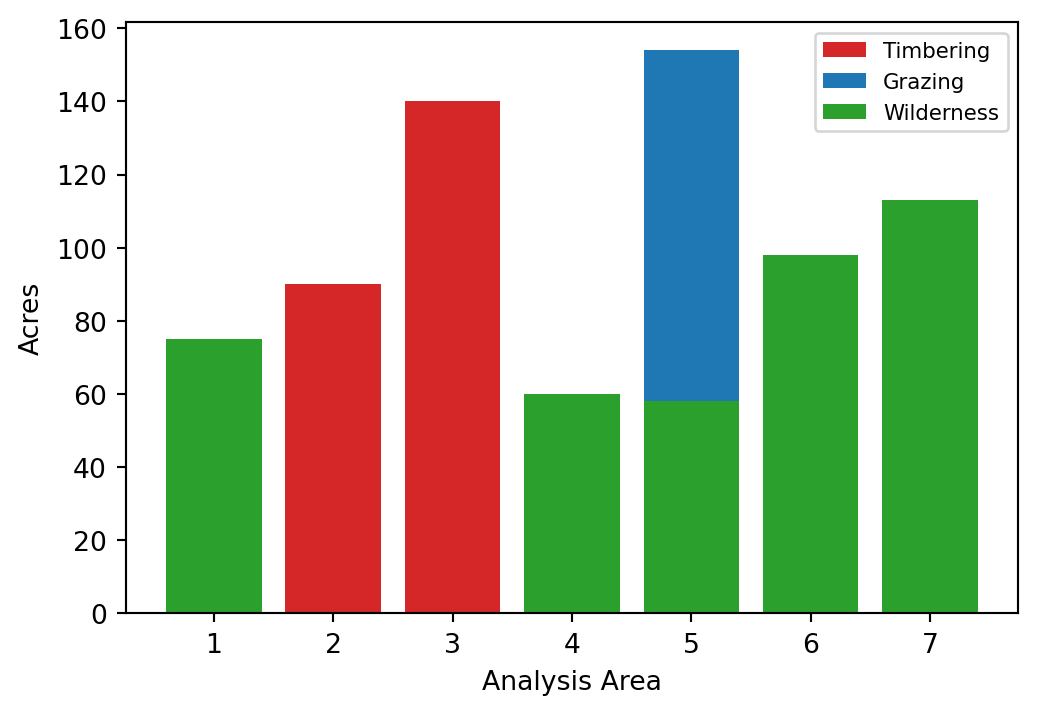
print("Area", i, "Prescription", j, ":", x[i,j].x, " acres")Area 1 Prescription 1 : 0.0 acres
Area 1 Prescription 2 : 0.0 acres
Area 1 Prescription 3 : 75.0 acres
Area 2 Prescription 1 : 90.0 acres
Area 2 Prescription 2 : 0.0 acres
Area 2 Prescription 3 : 0.0 acres
Area 3 Prescription 1 : 140.0 acres
Area 3 Prescription 2 : 0.0 acres
Area 3 Prescription 3 : 0.0 acres
Area 4 Prescription 1 : 0.0 acres
Area 4 Prescription 2 : 0.0 acres
Area 4 Prescription 3 : 60.0 acres
Area 5 Prescription 1 : 0.0 acres
Area 5 Prescription 2 : 153.99999999999966 acres
Area 5 Prescription 3 : 58.00000000000034 acres
Area 6 Prescription 1 : 0.0 acres
Area 6 Prescription 2 : 0.0 acres
Area 6 Prescription 3 : 98.0 acres
Area 7 Prescription 1 : 0.0 acres
Area 7 Prescription 2 : 0.0 acres
Area 7 Prescription 3 : 113.0 acresfig,ax = plt.subplots(figsize = (6,4))
colors = ['tab:red', 'tab:blue', 'tab:green']
for i in I:
for j in J:
ax.bar(i, x[i,j].x, color = colors[j-1])
ax.set_xlabel('Analysis Area')
ax.set_ylabel('Acres')
ax.legend(['Timbering', 'Grazing', 'Wilderness'], fontsize = 8)<matplotlib.legend.Legend at 0x22592fd9290>