── Conflicts ────────────────────────────────────────── tidyverse_conflicts() ──
✖ dplyr::filter() masks stats::filter()
✖ dplyr::lag()    masks stats::lag()
ℹ Use the conflicted package (<http://conflicted.r-lib.org/>) to force all conflicts to become errors
library(dplyr)library(nlme)
Attaching package: 'nlme'

The following object is masked from 'package:dplyr':

    collapse
library(lattice)library(ggplot2)library(plotrix)# Summarize the datatable(data$Tournament)
    Bundesliga         LaLiga        Ligue 1 Premier League        Serie A
            18             20             20             20             20
summary(data)
     Team            Tournament            Goals          Shots.pg
 Length:98          Length:98          Min.   :20.00   Min.   : 7.10
 Class :character   Class :character   1st Qu.:40.25   1st Qu.:10.32
 Mode  :character   Mode  :character   Median :50.00   Median :11.45
                                       Mean   :52.18   Mean   :11.85
                                       3rd Qu.:61.75   3rd Qu.:13.35
                                       Max.   :99.00   Max.   :17.10
  yellow_cards     red_cards       Possession.        Pass.
 Min.   : 40.0   Min.   : 0.000   Min.   :38.50   Min.   :66.50
 1st Qu.: 60.0   1st Qu.: 2.000   1st Qu.:46.23   1st Qu.:78.03
 Median : 67.5   Median : 3.000   Median :49.75   Median :80.80
 Mean   : 69.7   Mean   : 3.337   Mean   :50.00   Mean   :80.44
 3rd Qu.: 80.0   3rd Qu.: 4.750   3rd Qu.:52.85   3rd Qu.:83.45
 Max.   :117.0   Max.   :10.000   Max.   :62.40   Max.   :89.70
   AerialsWon        Rating
 Min.   : 9.50   Min.   :6.410
 1st Qu.:14.03   1st Qu.:6.540
 Median :16.10   Median :6.630
 Mean   :16.01   Mean   :6.646
 3rd Qu.:17.85   3rd Qu.:6.730
 Max.   :26.80   Max.   :7.010
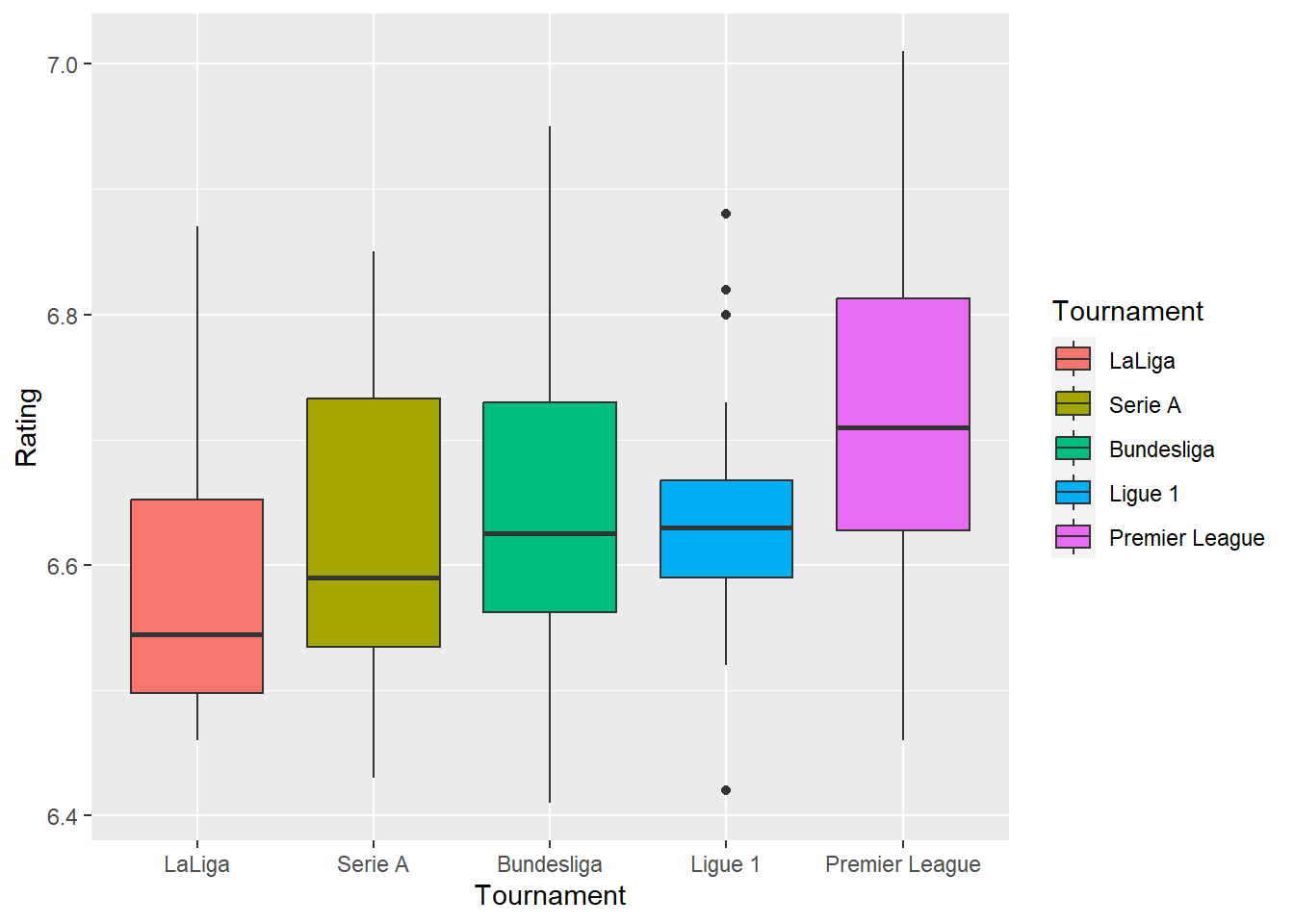
# Rating boxplotp <- data %>%mutate(Tournament =reorder(Tournament,Rating,FUN=median)) %>%ggplot(aes(Tournament,Rating,fill=Tournament))p +geom_boxplot()
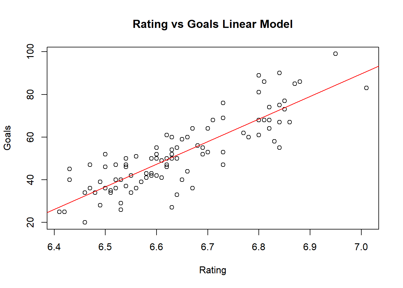
# Relationship between rating and other variables that has significant correlationplot(data$Rating,data$Goals,xlab="Rating",ylab="Goals",main ="Rating vs Goals Linear Model")abline(lm(Goals ~ Rating, data = data),col="red")
res<-lm(Goals ~ Rating, data = data)summary(res)
Call:
lm(formula = Goals ~ Rating, data = data)

Residuals:
    Min      1Q  Median      3Q     Max
-23.474  -4.882  -0.627   6.095  20.498

Coefficients:
            Estimate Std. Error t value Pr(>|t|)
(Intercept) -652.633     44.183  -14.77   <2e-16 ***
Rating       106.049      6.647   15.96   <2e-16 ***
---
Signif. codes:  0 '***' 0.001 '**' 0.01 '*' 0.05 '.' 0.1 ' ' 1

Residual standard error: 8.651 on 96 degrees of freedom
Multiple R-squared:  0.7262,    Adjusted R-squared:  0.7233
F-statistic: 254.6 on 1 and 96 DF,  p-value: < 2.2e-16
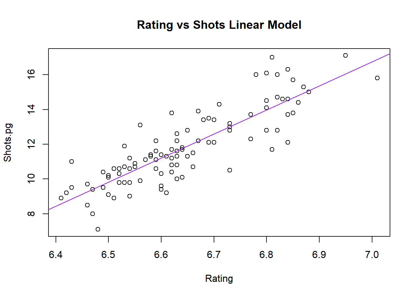
plot(data$Rating,data$Shots.pg, xlab="Rating",ylab="Shots.pg",main ="Rating vs Shots Linear Model")abline(lm(Shots.pg ~ Rating, data = data), col ="purple")
res3<-lm(Shots.pg ~ Rating, data = data)summary(res3)
Call:
lm(formula = Shots.pg ~ Rating, data = data)

Residuals:
     Min       1Q   Median       3Q      Max
-2.51255 -0.71796  0.04897  0.52414  2.87961

Coefficients:
            Estimate Std. Error t value Pr(>|t|)
(Intercept) -80.1841     5.7913  -13.85   <2e-16 ***
Rating       13.8479     0.8712   15.89   <2e-16 ***
---
Signif. codes:  0 '***' 0.001 '**' 0.01 '*' 0.05 '.' 0.1 ' ' 1

Residual standard error: 1.134 on 96 degrees of freedom
Multiple R-squared:  0.7247,    Adjusted R-squared:  0.7218
F-statistic: 252.7 on 1 and 96 DF,  p-value: < 2.2e-16
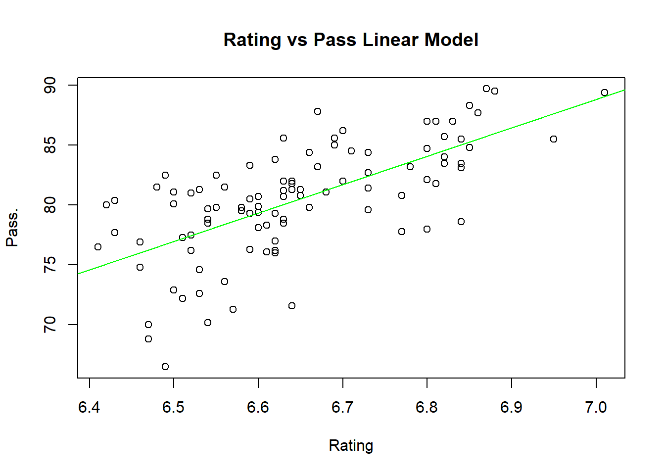
# Positive linear relationship between rating and both of these variables.plot(data$Rating,data$Pass., xlab="Rating",ylab="Pass.",main ="Rating vs Pass Linear Model")abline(lm(Pass. ~ Rating, data = data), col ="green")
res4<-lm(Pass. ~ Rating, data = data)summary(res4)
Call:
lm(formula = Pass. ~ Rating, data = data)

Residuals:
     Min       1Q   Median       3Q      Max
-10.2372  -1.8466   0.5051   2.3386   6.7916

Coefficients:
            Estimate Std. Error t value Pr(>|t|)
(Intercept)  -77.263     17.907  -4.315 3.88e-05 ***
Rating        23.729      2.694   8.809 5.38e-14 ***
---
Signif. codes:  0 '***' 0.001 '**' 0.01 '*' 0.05 '.' 0.1 ' ' 1

Residual standard error: 3.506 on 96 degrees of freedom
Multiple R-squared:  0.447, Adjusted R-squared:  0.4412
F-statistic:  77.6 on 1 and 96 DF,  p-value: 5.375e-14
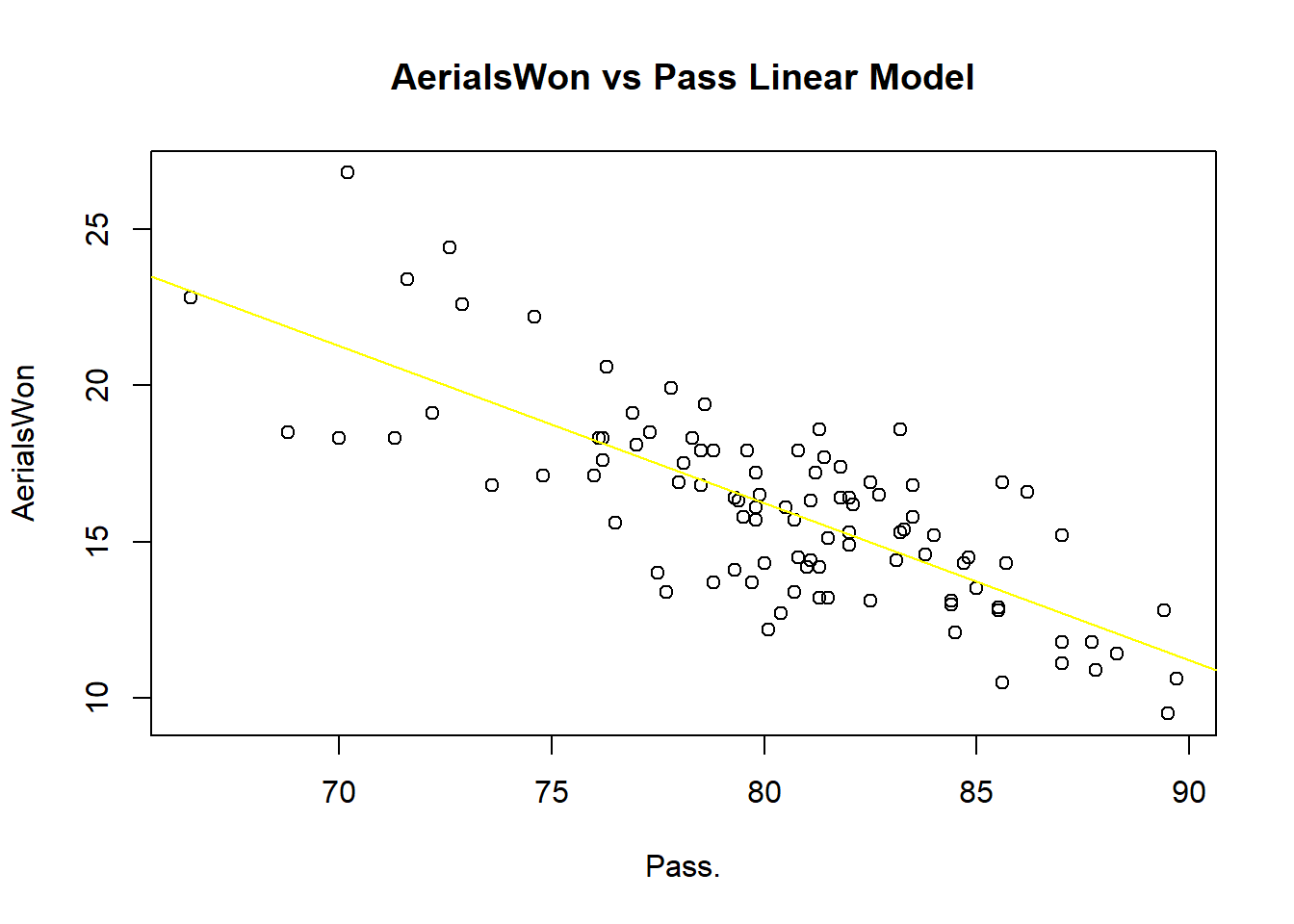
# Not as strongplot(data$Pass., data$AerialsWon, xlab ="Pass.", ylab ="AerialsWon", main ="AerialsWon vs Pass Linear Model")abline(lm(AerialsWon ~ Pass., data = data), col ="yellow")
res2 <-lm(AerialsWon ~ Pass., data = data)summary(res2)
Call:
lm(formula = AerialsWon ~ Pass., data = data)

Residuals:
    Min      1Q  Median      3Q     Max
-3.9827 -1.3630 -0.1802  1.2080  5.6519

Coefficients:
            Estimate Std. Error t value Pr(>|t|)
(Intercept) 56.39276    3.47829   16.21   <2e-16 ***
Pass.       -0.50206    0.04317  -11.63   <2e-16 ***
---
Signif. codes:  0 '***' 0.001 '**' 0.01 '*' 0.05 '.' 0.1 ' ' 1

Residual standard error: 1.994 on 96 degrees of freedom
Multiple R-squared:  0.5849,    Adjusted R-squared:  0.5806
F-statistic: 135.3 on 1 and 96 DF,  p-value: < 2.2e-16
# Negative linear relationship
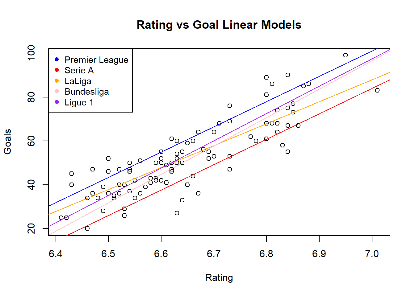
# Rating vs Goal comparison among tournamentsplot(data$Rating,data$Goals,xlab="Rating",ylab="Goals",main ="Rating vs Goal Linear Models")abline(lm(Goals ~ Rating, data =subset(data, Tournament =="Premier League")), col ="red")abline(lm(Goals ~ Rating, data =subset(data, Tournament =="Serie A")), col ="blue")abline(lm(Goals ~ Rating, data =subset(data, Tournament =="LaLiga")), col ="orange")abline(lm(Goals ~ Rating, data =subset(data, Tournament =="Bundesliga")), col ="pink")abline(lm(Goals ~ Rating, data =subset(data, Tournament =="Ligue 1")), col ="purple")legend("topleft",legend=c("Premier League","Serie A","LaLiga","Bundesliga","Ligue 1"),pch=16,cex =0.9, col=c("blue","red","orange","pink","purple"))
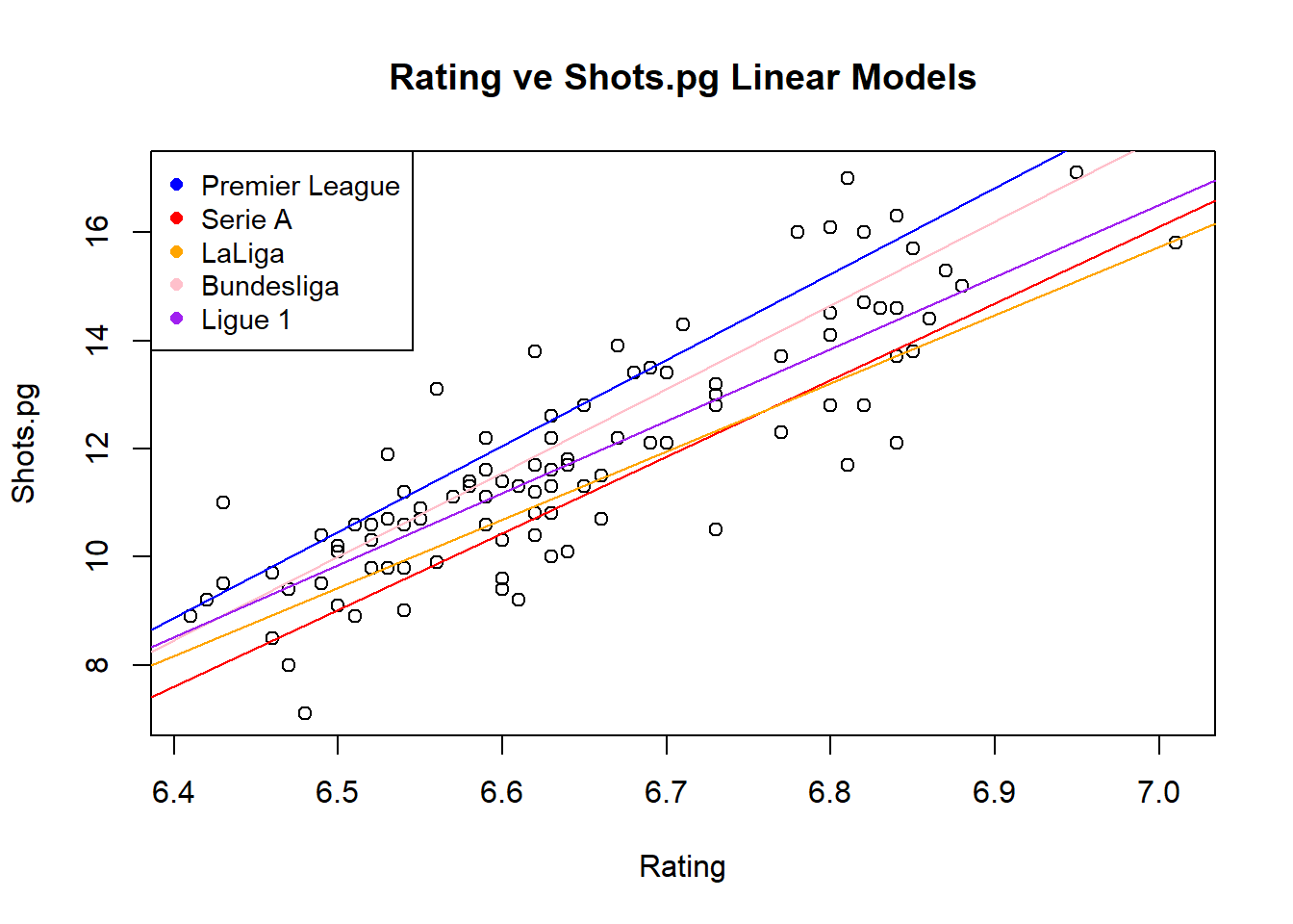
# Rating vs Shots comparison among tournamentsplot(data$Rating,data$Shots.pg,xlab="Rating",ylab="Shots.pg",main ="Rating ve Shots.pg Linear Models")abline(lm(Shots.pg ~ Rating, data =subset(data, Tournament =="Premier League")), col ="red")abline(lm(Shots.pg ~ Rating, data =subset(data, Tournament =="Serie A")), col ="blue")abline(lm(Shots.pg ~ Rating, data =subset(data, Tournament =="LaLiga")), col ="orange")abline(lm(Shots.pg ~ Rating, data =subset(data, Tournament =="Bundesliga")), col ="pink")abline(lm(Shots.pg ~ Rating, data =subset(data, Tournament =="Ligue 1")), col ="purple")legend("topleft",legend=c("Premier League","Serie A","LaLiga","Bundesliga","Ligue 1"),pch=16,cex =0.9, col=c("blue","red","orange","pink","purple"))
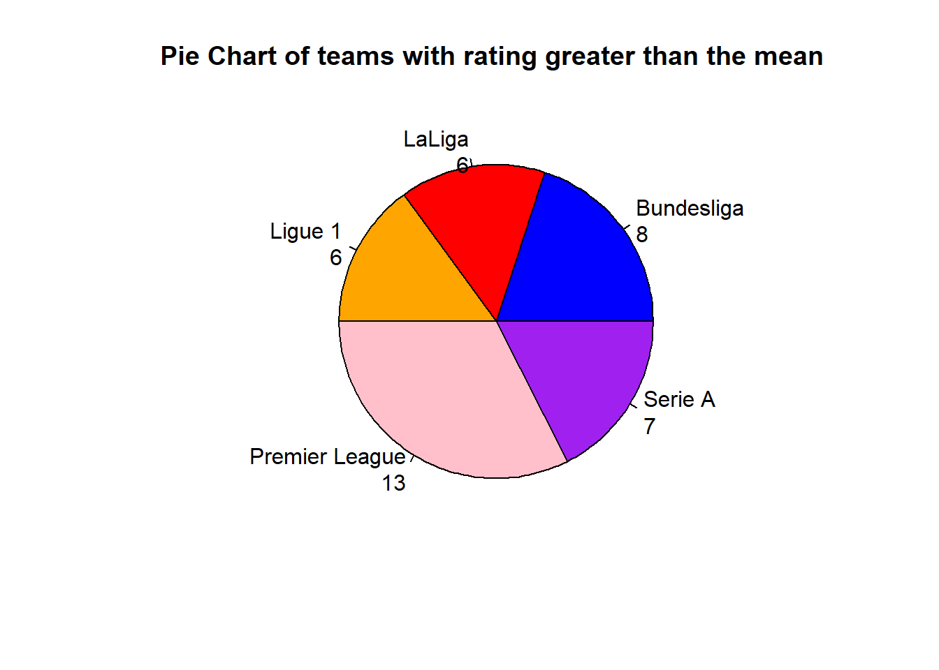
# First chart consists of the teams whose ratings are smaller than the average rating# in their specified tournament. Second chart consists of the teams whose ratings are greater than the average.up_group <- dplyr::filter(data,Rating>6.646)low_group <-dplyr::filter(data,Rating<6.646)mytable <-table(up_group$Tournament)lbls <-paste(names(mytable), "\n", mytable, sep="")pie(mytable, labels = lbls,main="Pie Chart of teams with rating greater than the mean ",col=c("blue","red","orange","pink","purple"))
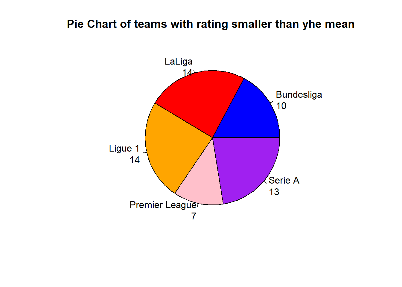
mytable <-table(low_group$Tournament)lbls <-paste(names(mytable), "\n", mytable, sep="")pie(mytable, labels = lbls,main="Pie Chart of teams with rating smaller than yhe mean ",col=c("blue","red","orange","pink","purple"))
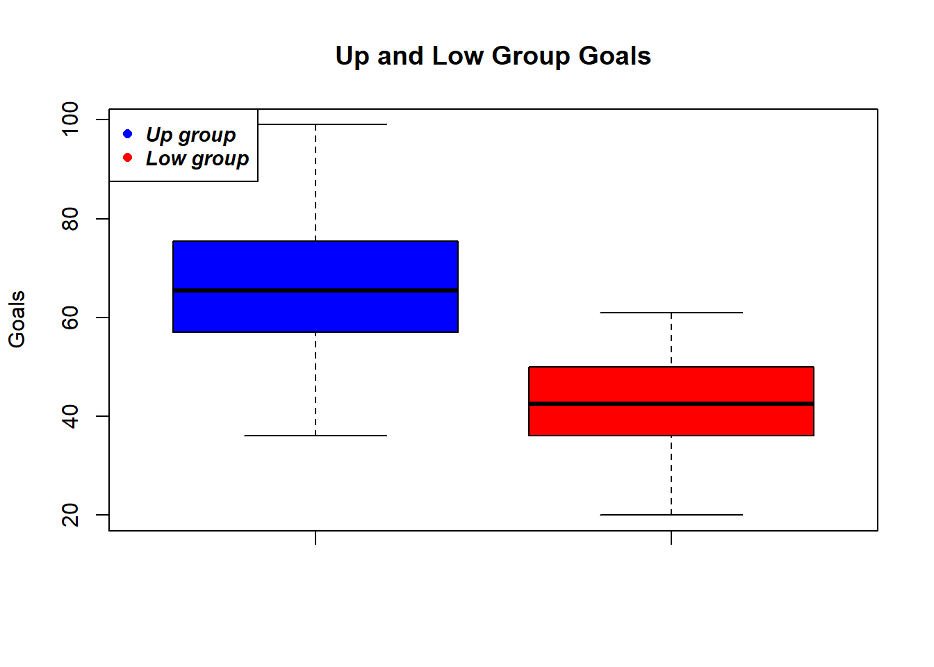
boxplot(up_group$Goals,low_group$Goals,ylab="Goals",main ="Up and Low Group Goals",col=c("blue","red"))legend("topleft", legend=c("Up group", "Low group"),pch=16,cex =0.9,col=c("blue", "red"), text.font=4)
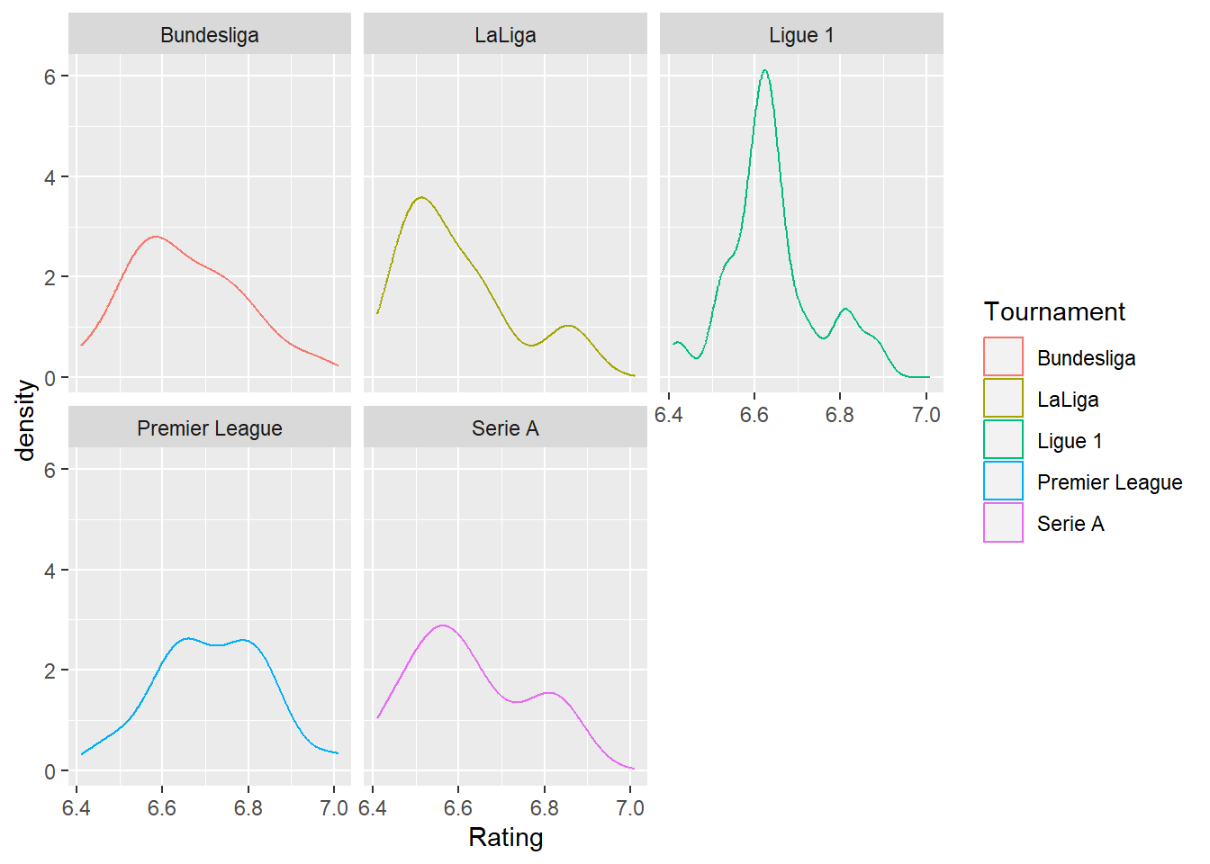
#Distributions of some variables faceted by Tournamentsdata %>%ggplot(aes(x=Rating, color=Tournament)) +geom_density() +facet_wrap(~Tournament)
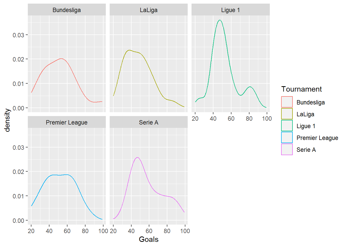
data %>%ggplot(aes(x=Goals, color=Tournament)) +geom_density() +facet_wrap(~Tournament)
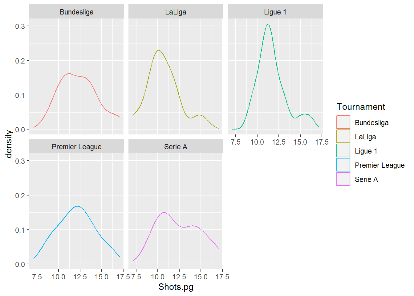
data %>%ggplot(aes(x=Shots.pg, color=Tournament)) +geom_density() +facet_wrap(~Tournament)
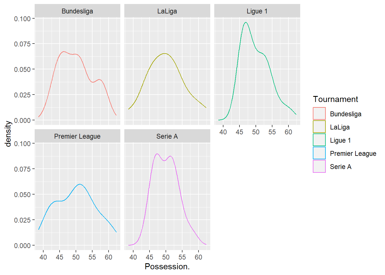
data %>%ggplot(aes(x=Possession., color=Tournament)) +geom_density() +facet_wrap(~Tournament)
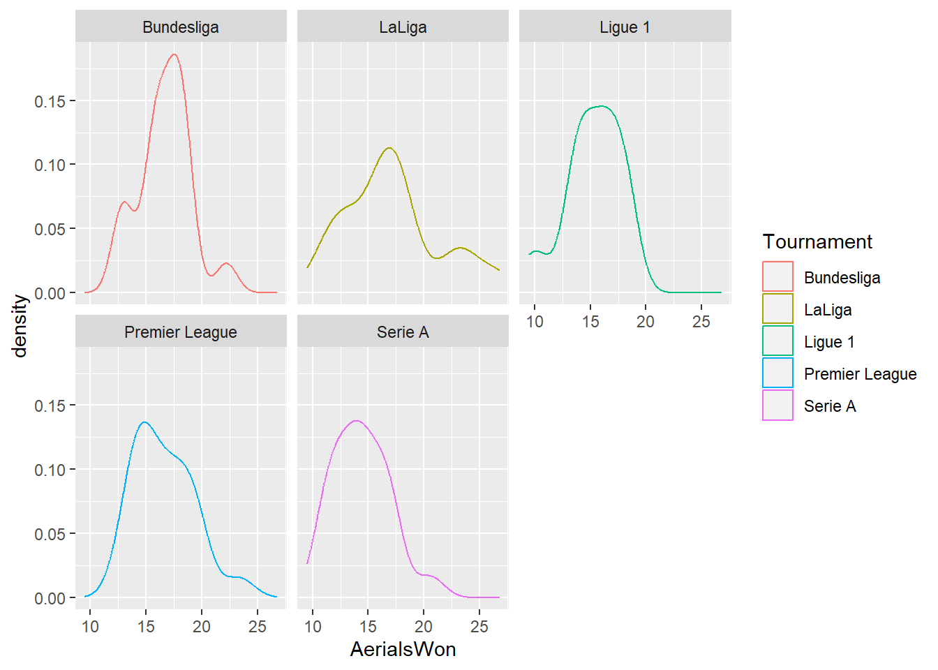
data %>%ggplot(aes(x=AerialsWon, color=Tournament)) +geom_density() +facet_wrap(~Tournament)