Analysis

About this site

This page involves the analysis part of our project.

Code

library(tidyverse)

── Attaching core tidyverse packages ──────────────────────── tidyverse 2.0.0 ──
✔ dplyr     1.1.4     ✔ readr     2.1.4
✔ forcats   1.0.0     ✔ stringr   1.5.0
✔ ggplot2   3.4.4     ✔ tibble    3.2.1
✔ lubridate 1.9.3     ✔ tidyr     1.3.0
✔ purrr     1.0.2     
── Conflicts ────────────────────────────────────────── tidyverse_conflicts() ──
✖ dplyr::filter() masks stats::filter()
✖ dplyr::lag()    masks stats::lag()
ℹ Use the conflicted package (<http://conflicted.r-lib.org/>) to force all conflicts to become errors

Code

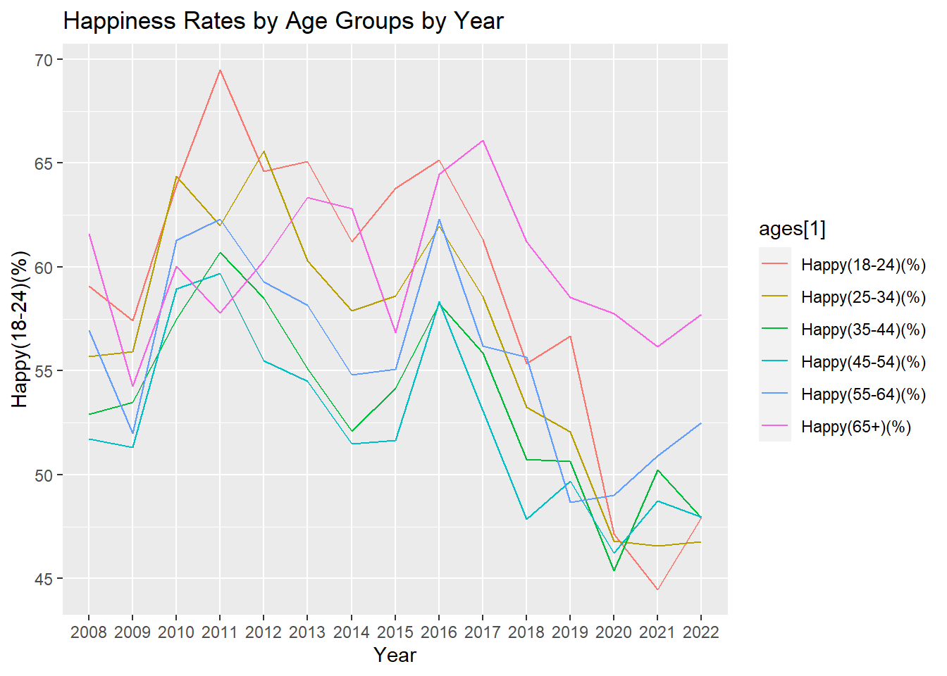
data <- get(load("final_data.RData"))
ages <- c("Happy(18-24)(%)","Happy(25-34)(%)","Happy(35-44)(%)","Happy(45-54)(%)","Happy(55-64)(%)","Happy(65+)(%)")
year_ages <- data |> select(Year, ages)

Warning: Using an external vector in selections was deprecated in tidyselect 1.1.0.
ℹ Please use `all_of()` or `any_of()` instead.
  # Was:
  data %>% select(ages)

  # Now:
  data %>% select(all_of(ages))

See <https://tidyselect.r-lib.org/reference/faq-external-vector.html>.

Code

year_ages

   Year Happy(18-24)(%) Happy(25-34)(%) Happy(35-44)(%) Happy(45-54)(%)
1  2008        59.09000        55.69000        52.90000        51.74000
2  2009        57.41000        55.92000        53.49000        51.31000
3  2010        63.93000        64.36000        57.49000        58.93000
4  2011        69.50000        62.00000        60.70000        59.70000
5  2012        64.60000        65.60000        58.50000        55.50000
6  2013        65.09000        60.29000        55.13000        54.49000
7  2014        61.20000        57.90000        52.10000        51.50000
8  2015        63.78700        58.60600        54.17800        51.66800
9  2016        65.13400        61.96100        58.22800        58.34400
10 2017        61.30150        58.57135        55.85570        53.08768
11 2018        55.35172        53.24284        50.74637        47.84929
12 2019        56.67982        52.04614        50.64638        49.70393
13 2020        47.14917        46.81024        45.37726        46.22153
14 2021        44.48447        46.57319        50.22658        48.75430
15 2022        47.90992        46.76606        47.93897        47.96122
   Happy(55-64)(%) Happy(65+)(%)
1         56.93000      61.60000
2         51.99000      54.27000
3         61.28000      60.03000
4         62.30000      57.80000
5         59.30000      60.30000
6         58.15000      63.36000
7         54.80000      62.80000
8         55.07000      56.84000
9         62.30000      64.47600
10        56.21379      66.09250
11        55.65419      61.19950
12        48.67123      58.54024
13        48.99747      57.74405
14        50.91547      56.16328
15        52.49462      57.72237

Code

ggplot(year_ages, aes(x = Year)) +
  geom_line(aes(y =`Happy(18-24)(%)`, color = ages[1], group=1)) +
  geom_line(aes(y =`Happy(25-34)(%)`, color = ages[2], group=1)) +
  geom_line(aes(y =`Happy(35-44)(%)`, color = ages[3], group=1)) +
  geom_line(aes(y =`Happy(45-54)(%)`, color = ages[4], group=1)) +
  geom_line(aes(y =`Happy(55-64)(%)`, color = ages[5], group=1)) +
  geom_line(aes(y =`Happy(65+)(%)`, color = ages[6], group=1)) +
  labs(title = "Happiness Rates by Age Groups by Year")

Code

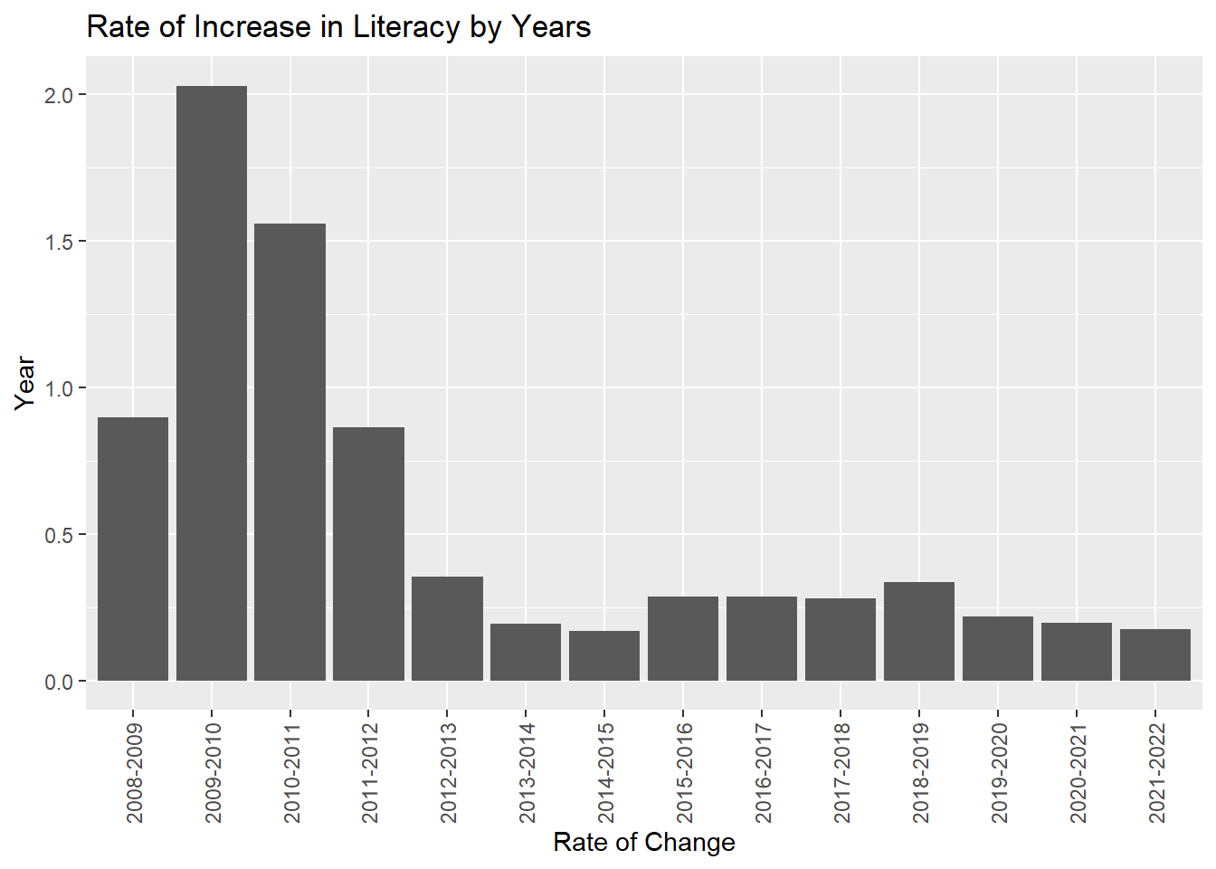
#GRAPH---2
rate_of_change <- c()

for (x in (1:14)) {
  ratio <- ((as.numeric(final_data[(x + 1), "Literate(%)"]) * 100) / as.numeric(final_data[x, "Literate(%)"])) - 100
  print(ratio)
  rate_of_change <- c(rate_of_change,ratio)
}

[1] 0.8991631
[1] 2.030331
[1] 1.559983
[1] 0.8646199
[1] 0.3549419
[1] 0.1920811
[1] 0.1695208
[1] 0.286889
[1] 0.2866629
[1] 0.2788856
[1] 0.335547
[1] 0.2194389
[1] 0.1966283
[1] 0.1742341

Code

rate_of_change

 [1] 0.8991631 2.0303310 1.5599834 0.8646199 0.3549419 0.1920811 0.1695208
 [8] 0.2868890 0.2866629 0.2788856 0.3355470 0.2194389 0.1966283 0.1742341

Code

x_axis = c("2008-2009","2009-2010","2010-2011","2011-2012","2012-2013","2013-2014","2014-2015","2015-2016","2016-2017","2017-2018","2018-2019","2019-2020","2020-2021","2021-2022")
mode(x_axis)

[1] "character"

Code

row_names <- c("rate_of_change", "x_axis")
df <- data.frame(rate_of_change, x_axis)

ggplot(df, aes(x = x_axis, y = as.numeric(rate_of_change))) + geom_col() +
  labs(title = "Rate of Increase in Literacy by Years") + 
  xlab("Rate of Change") + 
  ylab("Year") +
  theme(axis.text.x = element_text(angle = 90, vjust = 0.5, hjust=1))

Code

#GRAPH---3
data$`Happy(55-64)(%)`[9] <- 62.3001

happy_18_24_pop <- sapply(data$`Happy(18-24)(%)`, function(x) {x * data$`Pop(18-24)`[which(data$`Happy(18-24)(%)` == x)]})
happy_25_34_pop <- sapply(data$`Happy(25-34)(%)`, function(x) {x * data$`Pop(25-34)`[which(data$`Happy(25-34)(%)` == x)]})
happy_35_44_pop <- sapply(data$`Happy(35-44)(%)`, function(x) {x * data$`Pop(35-44)`[which(data$`Happy(35-44)(%)` == x)]})
happy_45_54_pop <- sapply(data$`Happy(45-54)(%)`, function(x) {x * data$`Pop(45-54)`[which(data$`Happy(45-54)(%)` == x)]})
happy_55_64_pop <- sapply(data$`Happy(55-64)(%)`, function(x) {x * data$`Pop(55-64)`[which(data$`Happy(55-64)(%)` == x)]})
happy_65_pop <- sapply(data$`Happy(65+)(%)`, function(x) {x * data$`Pop(65+)`[which(data$`Happy(65+)(%)` == x)]})

happy_pop_df <- data.frame(happy_18_24_pop, happy_25_34_pop, happy_35_44_pop, happy_45_54_pop, happy_55_64_pop, happy_65_pop)
happy_pop_total_df <- happy_pop_df |> mutate(Total_Happy = rowSums(happy_pop_df))


happy_pop_total_ratio <- sapply(as.numeric(happy_pop_total_df$Total_Happy), function(x) {x / as.numeric(data$`Pop(Total)`[which(happy_pop_total_df$Total_Happy == x)])})
print(happy_pop_total_ratio)

 [1] 38.24621 37.41853 42.42036 43.33331 42.70288 41.59463 39.83181 40.27278
 [9] 43.78367 41.59795 38.40338 37.92216 35.04362 36.03976 36.52276

Code

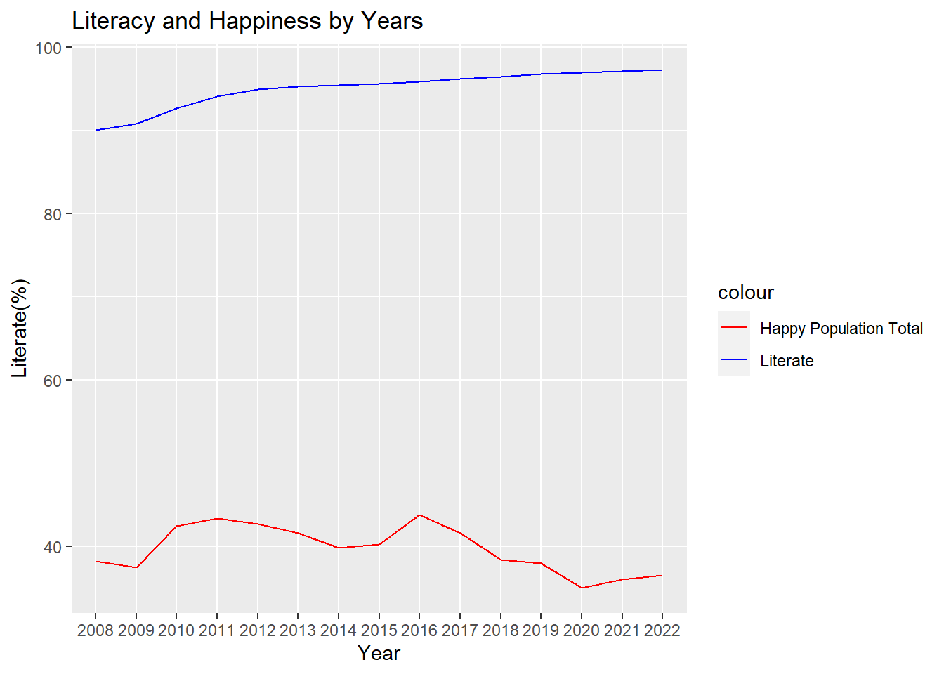
ggplot(data, aes(x = Year)) +
    geom_line(aes(y = as.numeric(`Literate(%)`), color = "red", group=2)) +
  geom_line(aes(y = happy_pop_total_ratio, color = "blue", group=1)) + 
  labs(title = "Literacy and Happiness by Years") + ylab("Literate(%)") +
  scale_color_manual(values = c("red", "blue"),
                     labels = c("Happy Population Total","Literate"))

Code

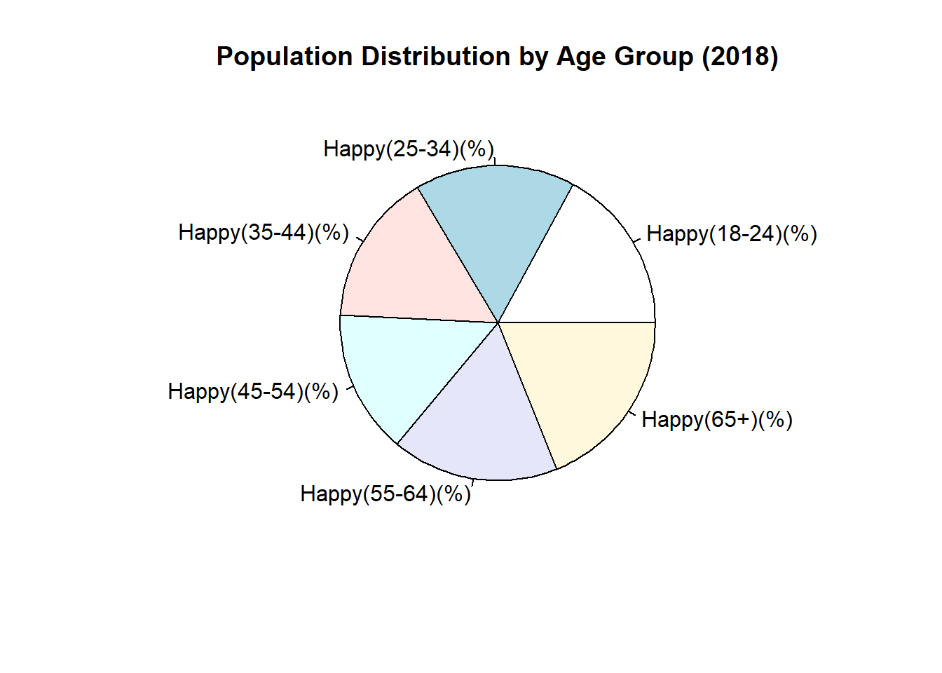
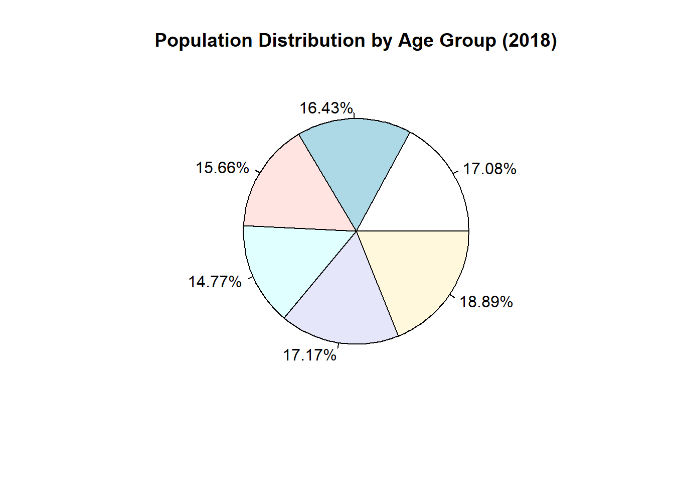
#Pie Plot

happiness_percentages <- data[11, c("Happy(18-24)(%)", "Happy(25-34)(%)", "Happy(35-44)(%)", 
                                    "Happy(45-54)(%)", "Happy(55-64)(%)", "Happy(65+)(%)")]

actual_populations <- as.numeric(happiness_percentages)

pie(actual_populations, labels = (c("Happy(18-24)(%)", "Happy(25-34)(%)", "Happy(35-44)(%)","Happy(45-54)(%)", "Happy(55-64)(%)", "Happy(65+)(%)")), main = "Population Distribution by Age Group (2018)")

Code

pie_labels <- paste0(round(100 * happiness_percentages/sum(happiness_percentages), 2), "%")

pie(actual_populations, labels = pie_labels , main = "Population Distribution by Age Group (2018)")

Code

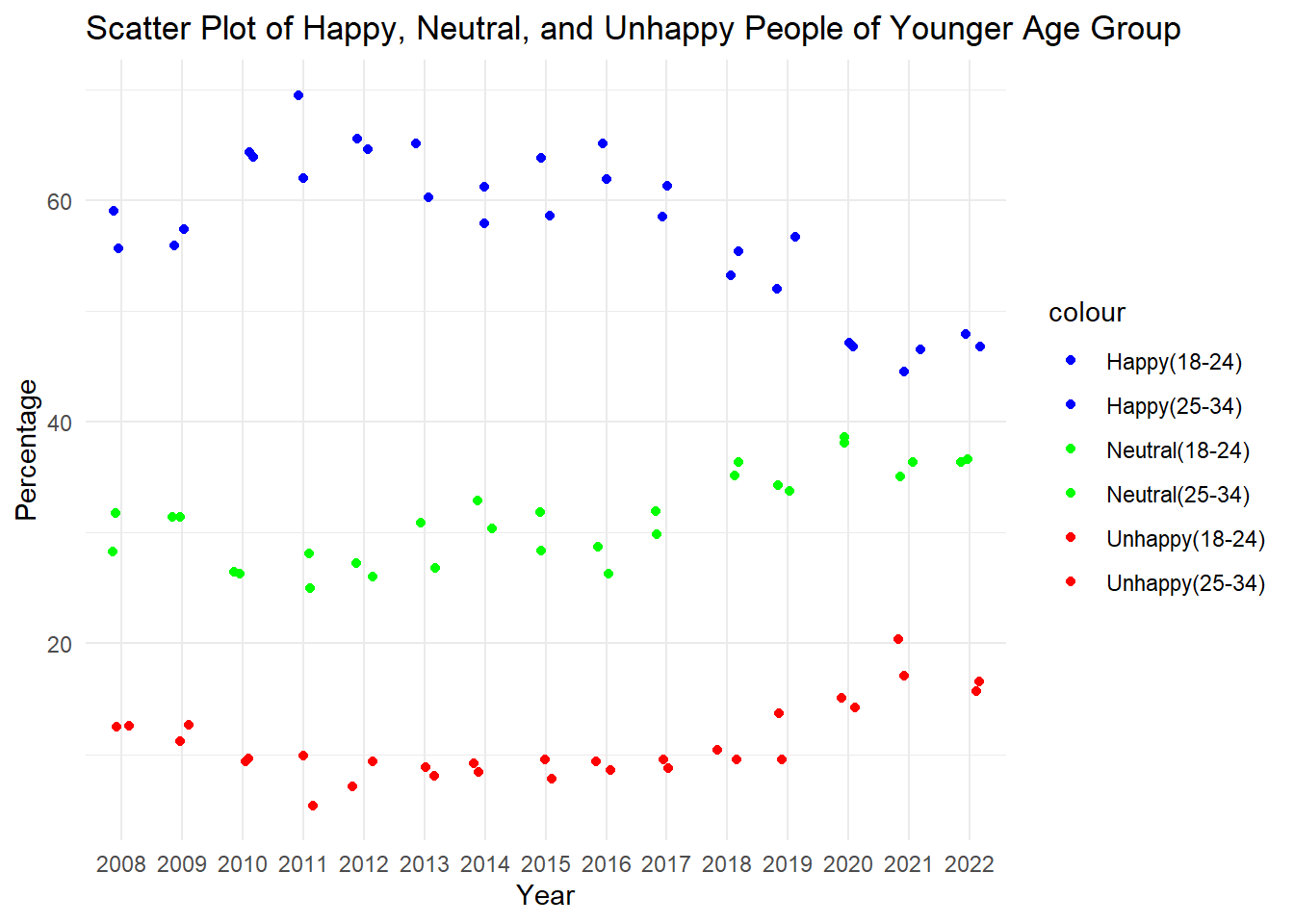
library(ggplot2)
your_data <- get(load('testing_data.RData'))

ggplot(your_data, aes(x = Year)) +
  geom_point(aes(y = `Happy(18-24)(%)`, color = "Happy(18-24)"), position = position_jitter(width = 0.2)) +
  geom_point(aes(y = `Neutral(18-24)(%)`, color = "Neutral(18-24)"), position = position_jitter(width = 0.2)) +
  geom_point(aes(y = `Unhappy(18-24)(%)`, color = "Unhappy(18-24)"), position = position_jitter(width = 0.2)) +
  geom_point(aes(y = `Happy(25-34)(%)`, color = "Happy(25-34)"), position = position_jitter(width = 0.2)) +
  geom_point(aes(y = `Neutral(25-34)(%)`, color = "Neutral(25-34)"), position = position_jitter(width = 0.2)) +
  geom_point(aes(y = `Unhappy(25-34)(%)`, color = "Unhappy(25-34)"), position = position_jitter(width = 0.2)) +



  labs(title = "Scatter Plot of Happy, Neutral, and Unhappy People of Younger Age Group",
       x = "Year",
       y = "Percentage") +
  scale_color_manual(values = c("Happy(18-24)" = "blue", "Neutral(18-24)" = "green", "Unhappy(18-24)" = "red",
                                "Happy(25-34)" = "blue", "Neutral(25-34)" = "green", "Unhappy(25-34)" = "red")) +
  theme_minimal()

Code

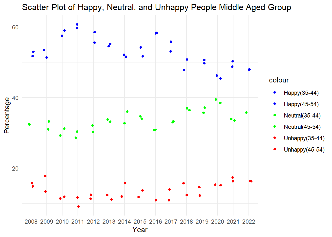
 library(ggplot2)
your_data <- get(load('testing_data.RData'))

ggplot(your_data, aes(x = Year)) +
  geom_point(aes(y = `Happy(35-44)(%)`, color = "Happy(35-44)"), position = position_jitter(width = 0.2)) +
  geom_point(aes(y = `Neutral(35-44)(%)`, color = "Neutral(35-44)"), position = position_jitter(width = 0.2)) +
  geom_point(aes(y = `Unhappy(35-44)(%)`, color = "Unhappy(35-44)"), position = position_jitter(width = 0.2)) +
  geom_point(aes(y = `Happy(45-54)(%)`, color = "Happy(45-54)"), position = position_jitter(width = 0.2)) +
  geom_point(aes(y = `Neutral(45-54)(%)`, color = "Neutral(45-54)"), position = position_jitter(width = 0.2)) +
  geom_point(aes(y = `Unhappy(45-54)(%)`, color = "Unhappy(45-54)"), position = position_jitter(width = 0.2)) +

  labs(title = "Scatter Plot of Happy, Neutral, and Unhappy People Middle Aged Group",
       x = "Year",
       y = "Percentage") +
  scale_color_manual(values = c("Happy(35-44)" = "blue", "Neutral(35-44)" = "green", "Unhappy(35-44)" = "red",
                                "Happy(45-54)" = "blue", "Neutral(45-54)" = "green", "Unhappy(45-54)" = "red")) +
  theme_minimal()

Code

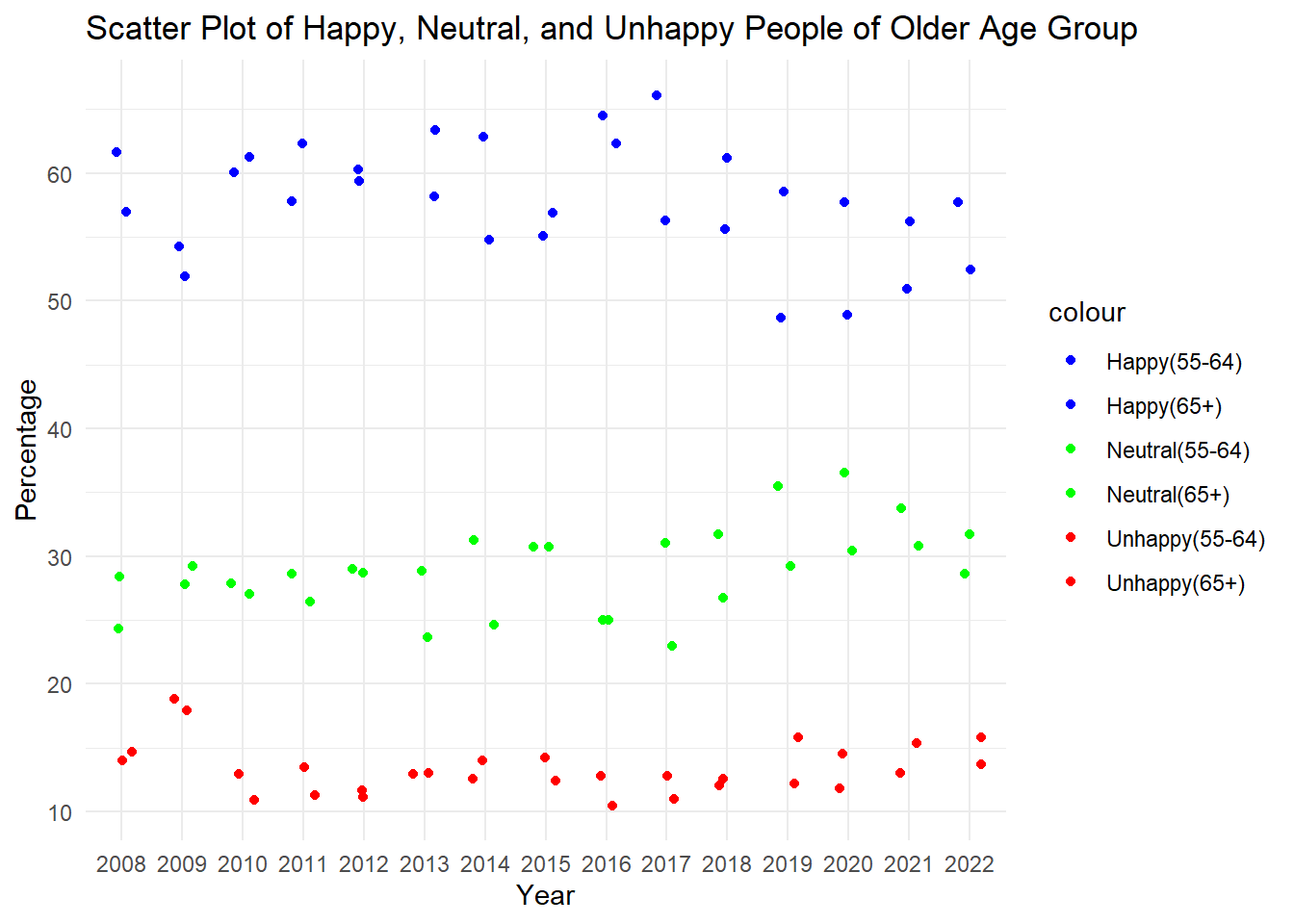
library(ggplot2)
your_data <- get(load('testing_data.RData'))

ggplot(your_data, aes(x = Year)) +
  geom_point(aes(y = `Happy(55-64)(%)`, color = "Happy(55-64)"), position = position_jitter(width = 0.2)) +
  geom_point(aes(y = `Neutral(55-64)(%)`, color = "Neutral(55-64)"), position = position_jitter(width = 0.2)) +
  geom_point(aes(y = `Unhappy(55-64)(%)`, color = "Unhappy(55-64)"), position = position_jitter(width = 0.2)) +
  geom_point(aes(y = `Happy(65+)(%)`, color = "Happy(65+)"), position = position_jitter(width = 0.2)) +
  geom_point(aes(y = `Neutral(65+)(%)`, color = "Neutral(65+)"), position = position_jitter(width = 0.2)) +
  geom_point(aes(y = `Unhappy(65+)(%)`, color = "Unhappy(65+)"), position = position_jitter(width = 0.2)) +

  labs(title = "Scatter Plot of Happy, Neutral, and Unhappy People of Older Age Group",
       x = "Year",
       y = "Percentage") +
  scale_color_manual(values = c("Happy(55-64)" = "blue", "Neutral(55-64)" = "green", "Unhappy(55-64)" = "red",
                                "Happy(65+)" = "blue", "Neutral(65+)" = "green", "Unhappy(65+)" = "red")) +
  theme_minimal()

Code

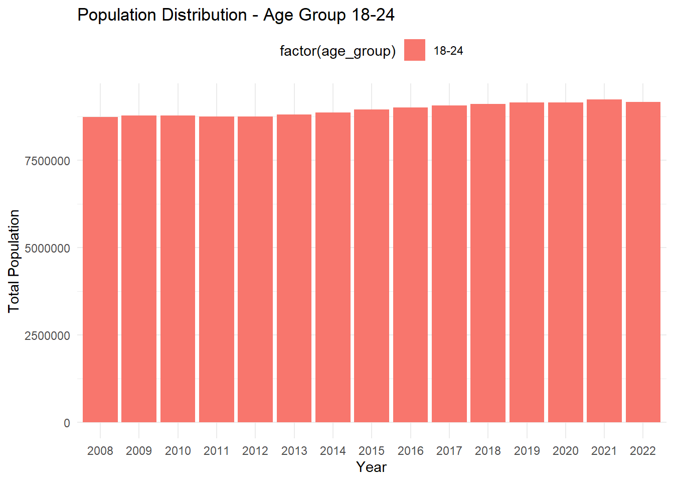
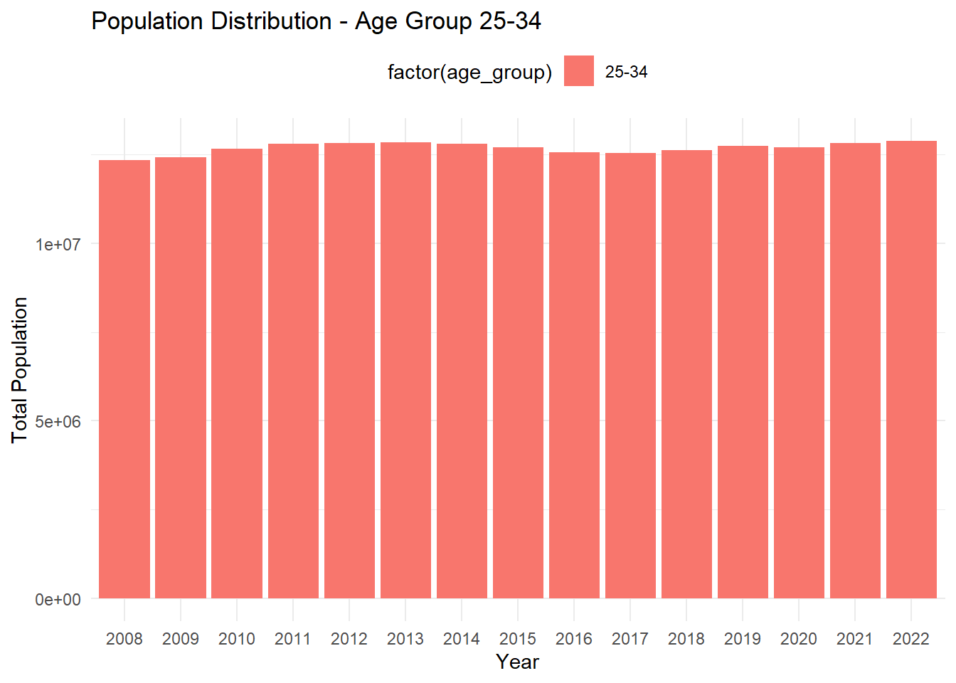
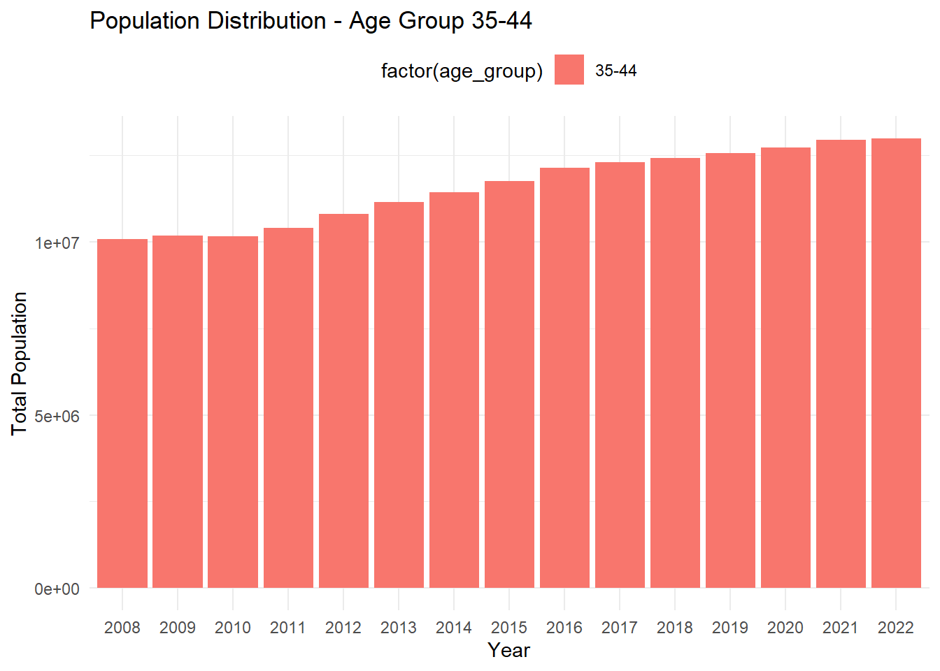
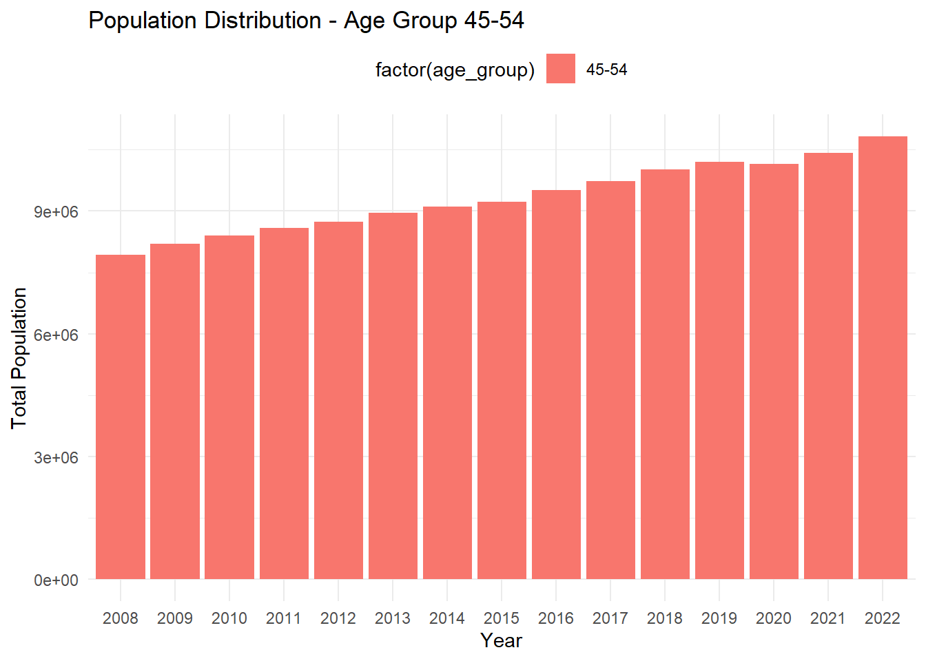
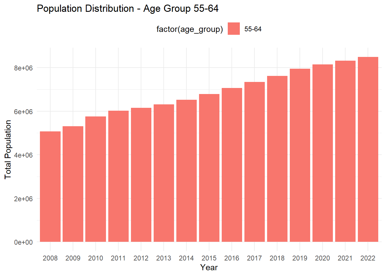
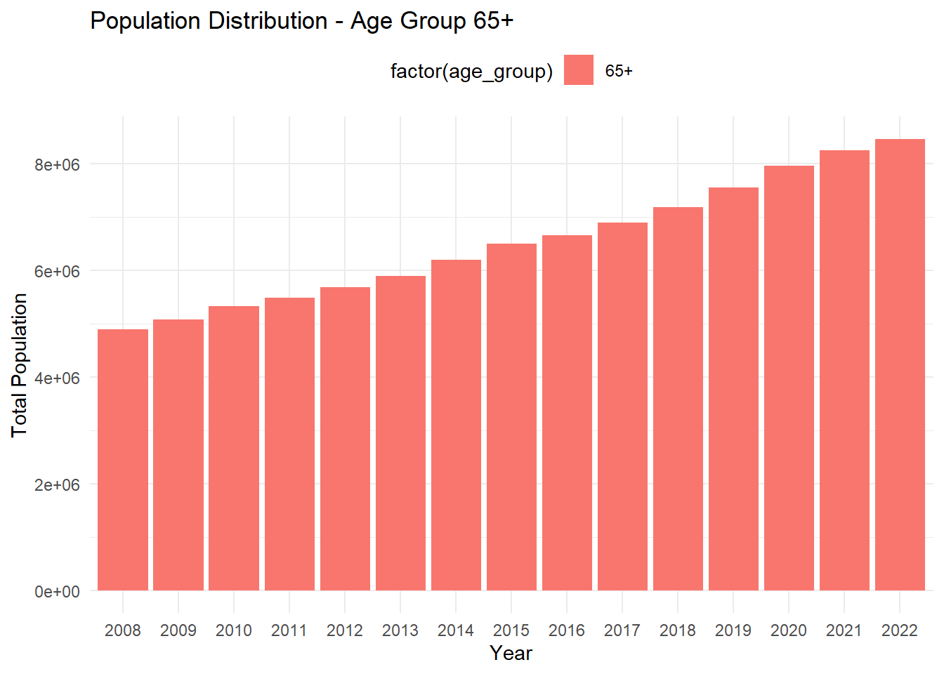
library(ggplot2)


your_data <- get(load('testing_data.RData'))

age_groups <- c("18-24", "25-34", "35-44", "45-54", "55-64", "65+")


plots_list <- list()


for (age_group in age_groups) {

  age_group_columns <- grep(paste0("(", age_group, ")"), colnames(your_data), value = TRUE)
  

  plot <- ggplot(your_data, aes(x = Year)) +
    geom_bar(aes(y = get(paste0("Pop","(", age_group,")")), fill = factor(age_group)),
             stat = "identity", position = "stack") +
    labs(title = paste("Population Distribution - Age Group", age_group),
         x = "Year",
         y = "Total Population") +
    theme_minimal() +
    theme(legend.position = "top")
  

  plots_list[[age_group]] <- plot
}


for (age_group in age_groups) {
  print(plots_list[[age_group]])
}

Code

library(corrplot)

corrplot 0.92 loaded

Code

your_data <- get(load('testing_data.RData'))

selected_columns <- c("Literate(%)", "Illiterate(%)", "Pop(Total)",
                       "Pop(18-24)", "Pop(25-34)", "Pop(35-44)",
                       "Pop(45-54)", "Pop(55-64)", "Pop(65+)",
                       "Happy(18-24)(%)", "Neutral(18-24)(%)", "Unhappy(18-24)(%)",
                       "Happy(25-34)(%)", "Neutral(25-34)(%)", "Unhappy(25-34)(%)",
                       "Happy(35-44)(%)", "Neutral(35-44)(%)", "Unhappy(35-44)(%)",
                       "Happy(45-54)(%)", "Neutral(45-54)(%)", "Unhappy(45-54)(%)",
                       "Happy(55-64)(%)", "Neutral(55-64)(%)", "Unhappy(55-64)(%)",
                       "Happy(65+)(%)", "Neutral(65+)(%)", "Unhappy(65+)(%)")


selected_data <- your_data[, selected_columns]

selected_data[] <- lapply(selected_data, function(x) as.numeric(as.character(x)))


correlation_matrix <- cor(selected_data, use = "complete.obs")

corrplot(correlation_matrix, method = "color", type = "upper", tl.col = "black", tl.srt = 45)

Code

library(ggplot2)

your_data <- get(load('testing_data.RData'))


library(reshape2)

Attaching package: 'reshape2'

The following object is masked from 'package:tidyr':

    smiths

Code

melted_data <- melt(your_data, id.vars = c("Year"), measure.vars = c(
  "Happy(18-24)(%)", "Neutral(18-24)(%)", "Unhappy(18-24)(%)",
  "Happy(25-34)(%)", "Neutral(25-34)(%)", "Unhappy(25-34)(%)",
  "Happy(35-44)(%)", "Neutral(35-44)(%)", "Unhappy(35-44)(%)",
  "Happy(45-54)(%)", "Neutral(45-54)(%)", "Unhappy(45-54)(%)",
  "Happy(55-64)(%)", "Neutral(55-64)(%)", "Unhappy(55-64)(%)",
  "Happy(65+)(%)", "Neutral(65+)(%)", "Unhappy(65+)(%)"
))


ggplot(melted_data, aes(x = variable, y = value, fill = variable)) +
  geom_boxplot() +
  labs(title = "Boxplots for Happiness Levels Across Age Groups",
       x = "Age Group",
       y = "Percentage",
       fill = "Happiness Level") +
  theme_minimal() +
  theme(axis.text.x = element_text(angle = 45, hjust = 1))