ANALYSIS

KEY TAKEAWAYS

The aim of this project is to analyze internal migration data in Turkey and investigate the factors such as migration reasons, age, education, and other variables that influence migration. We conducted our research using the internal migration and population datasets available on the Turkish Statistical Institute (TÜİK) website. The conclusions drawn from this project are outlined in the following points:

1. We had assumed that the highest migration due to retirement would be to the Central Anatolia Region or the Aegean Region. To validate this assumption, we created a migration value and cause graph. When looking at this graph, we observed that the highest migration is to the Marmara Region. To obtain more accurate results, we created a migration rate and cause graph. In this graph, we see that the highest migration is to the Black Sea and Aegean regions. So, we realized that part of our assumption is correct. Understanding the importance of creating a Rate graph, we concluded that we should make decisions based on this graph.

2. The age range of the people who migrate the most is seen in the graph as 20-24. The age group of the people who migrated the second most is seen in the graph as 15-19. In the graph of reasons for migration, the most common reason for migration was observed to be education. We can reconcile this incident with this situation.

3. The visual representation of migration numbers across different educational backgrounds highlights a compelling inverse relationship between education and migration. Doctoral and primary school-educated individuals show lower migration rates compared to high school and university-educated individuals. Individuals with higher education levels tend to migrate less. The scatter plot analysis reveals a lack of a straightforward correlation between the average education level and fertility rates across regions in the dataset. While some general trends emerge like higher education levels in certain regions coinciding with lower fertility rates outliers such as Central Anatolia and the Mediterranean Region defy these patterns.

4. TÜİK has divided provinces into 26 regions based on geographical proximity, simplifying regional oversight and data collection as cities in these regions are closely clustered. The graph comparing workforce to usable income generally shows an increase in usable income as the workforce increases, yet this trend varies among regions. Additionally, the Usable Income data is calculated based on the Gini coefficient. The Gini coefficient, in turn, represents the distribution of usable income within a region. For example, according to 2021 TÜİK data, Istanbul’s Gini coefficient of 0.43 compared to Izmir’s 0.37 indicates a higher income inequality in Istanbul.

DATA PREPROCESSING

Click the see the code

# importing necessary packages
library(tidyverse)
library(readxl)
library(readr)
library(gridExtra)
library(dplyr)

population <- read_excel("C:\\Users\\melike\\desktop\\DataVizards_FinalDataFrame.xlsx")
names(population) <- c('IDD','city','regionid','regions','totalpop','male','female','age04','age59','age1014','age1519','age2024','age2529','age3034','age3539','age4044','otherage','unknowns','doctorate','primaryedu','elementaryedu','highschool','literatebutnoschool','notliterate','middleschool','master','university','fertilityrate','electricity','numberofattempts','housingsalesnumbers')

region26 <- read_excel("C:\\Users\\melike\\desktop\\DataVizards_FinalDataFrame.xlsx", sheet = "Bolge26")
names(region26) <- c('region','region2id','workforce15plus','workforce1564','usableincome')

migration <- read_excel("C:\\Users\\melike\\desktop\\DataVizards_FinalDataFrame.xlsx")
population <- read_excel("C:\\Users\\melike\\desktop\\DataVizards_FinalDataFrame.xlsx")
names(population) <- c('IDD','city','regionid','regions','totalpop','male','female','age04','age59','age1014','age1519','age2024','age2529','age3034','age3539','age4044','otherage','unknowns','doctorate','primaryedu','elementaryedu','highschool','literatebutnoschool','notliterate','middleschool','master','university','fertilityrate','electricity','numberofattempts','housingsalesnumbers')

region26 <- read_excel("C:\\Users\\melike\\desktop\\DataVizards_FinalDataFrame.xlsx", sheet = "Bolge26")
names(region26) <- c('region','region2id','workforce15plus','workforce1564','usableincome')

migration <- read_excel("C:\\Users\\melike\\desktop\\DataVizards_FinalDataFrame.xlsx", sheet = "Goc Bilgileri")

population <- read_excel("C:\\Users\\melike\\desktop\\DataVizards_FinalDataFrame.xlsx")
names(population) <- c('IDD','city','regionid','regions','totalpop','male','female','age04','age59','age1014','age1519','age2024','age2529','age3034','age3539','age4044','otherage','unknowns','doctorate','primaryedu','elementaryedu','highschool','literatebutnoschool','notliterate','middleschool','master','university','fertilityrate','electricity','numberofattempts','housingsalesnumbers')

region26 <- read_excel("C:\\Users\\melike\\desktop\\DataVizards_FinalDataFrame.xlsx", sheet = "Bolge26")
names(region26) <- c('region','region2id','workforce15plus','workforce1564','usableincome')

migration <- read_excel("C:\\Users\\melike\\desktop\\DataVizards_FinalDataFrame.xlsx", sheet = "Goc Bilgileri")

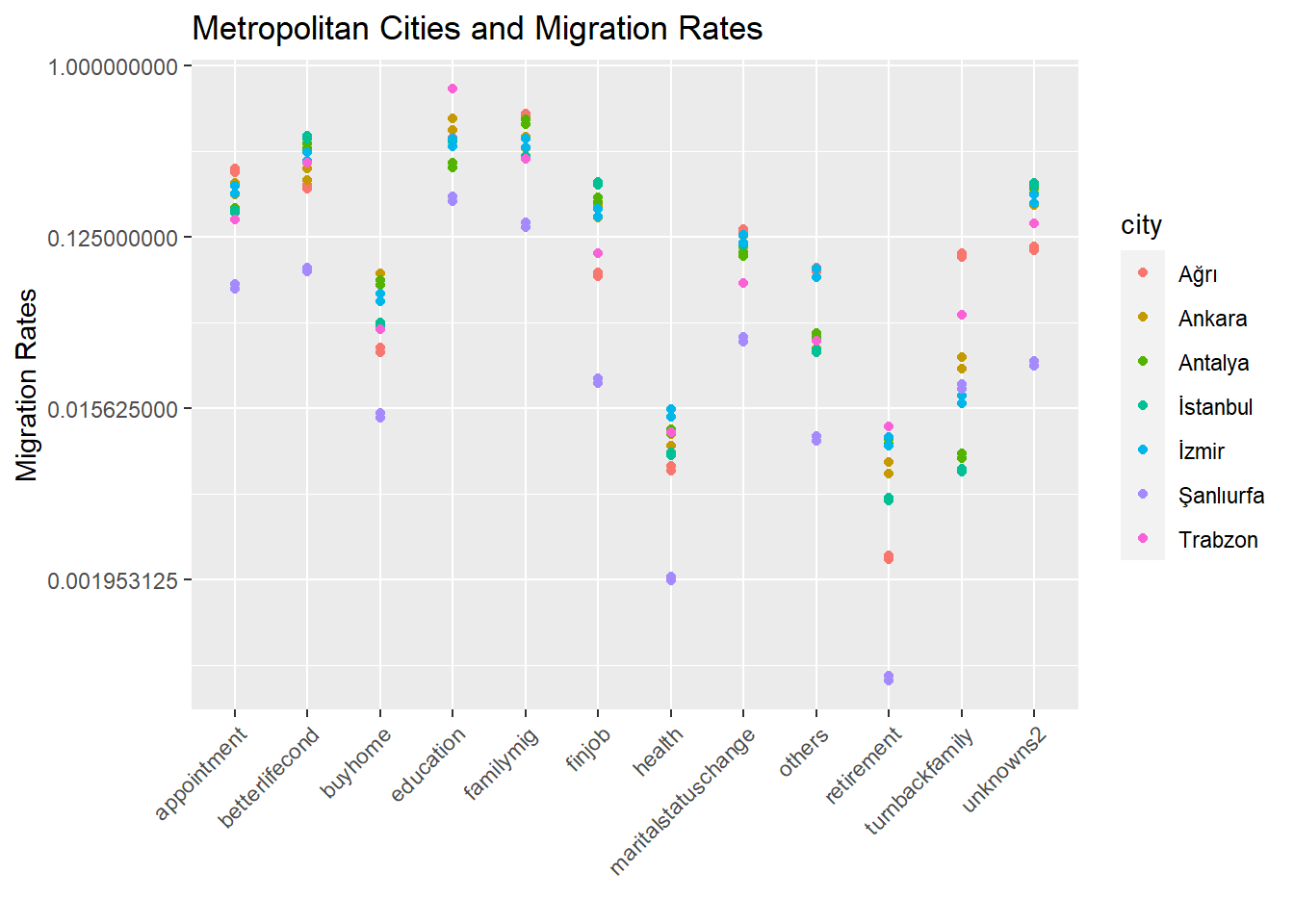
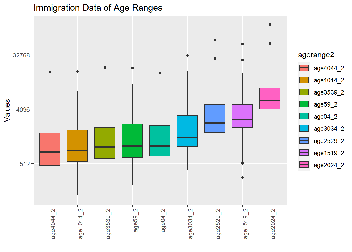
names(migration) <- c('IDD','male2','female2','turnbackfamily','unknowns2','betterlifecond','others','education','retirement','buyhome','familymig','finjob','maritalstatuschange','health','appointment','age04_2','age59_2','age1014_2','age1519_2','age2024_2','age2529_2','age3034_2','age3539_2','age4044_2','university2','highschool2','middleschool2', 'elementaryschool2')


# tidy migration dataset
migration$city <- population$city 
migration$regions <- population$regions

tidy_data_gender <- migration |> pivot_longer(c(male2,female2),names_to = "gender2",values_to = "gender_value2")


tidy_data_causes <- tidy_data_gender |> pivot_longer(c(turnbackfamily,unknowns2,betterlifecond,others,education,
                                                retirement,buyhome,familymig,finjob,maritalstatuschange,health,appointment),names_to = "migrationcauses",values_to = "migrationcauses_value")

tidy_data_age <- tidy_data_causes |> pivot_longer(c(age04_2,age59_2,age1014_2,age1519_2,
                                                    age2024_2,age2529_2,age3034_2,age3539_2,age4044_2),names_to = "agerange2",values_to = "agerange_value2")

last_migration_tidy_data <- tidy_data_age |> pivot_longer(c(university2,highschool2,middleschool2,elementaryschool2),names_to = "education2",values_to = "education_value2")
head(last_migration_tidy_data)

# A tibble: 6 × 11
    IDD city  regions         gender2 gender_value2 migrationcauses
  <dbl> <chr> <chr>           <chr>           <dbl> <chr>          
1     1 Adana Akdeniz Bölgesi male2           25200 turnbackfamily 
2     1 Adana Akdeniz Bölgesi male2           25200 turnbackfamily 
3     1 Adana Akdeniz Bölgesi male2           25200 turnbackfamily 
4     1 Adana Akdeniz Bölgesi male2           25200 turnbackfamily 
5     1 Adana Akdeniz Bölgesi male2           25200 turnbackfamily 
6     1 Adana Akdeniz Bölgesi male2           25200 turnbackfamily 
# ℹ 5 more variables: migrationcauses_value <dbl>, agerange2 <chr>,
#   agerange_value2 <dbl>, education2 <chr>, education_value2 <dbl>

Click the see the code

# tidy region26 dataset
tidy_region26 <- region26 |> pivot_longer(c(workforce15plus,workforce1564),names_to = "workforce",values_to = "workforce_values")
head(tidy_region26)

# A tibble: 6 × 5
  region                     region2id usableincome workforce   workforce_values
  <chr>                      <chr>            <dbl> <chr>                  <dbl>
1 Adana, Mersin              TR62             0.382 workforce1…             1579
2 Adana, Mersin              TR62             0.382 workforce1…             1528
3 Ağrı, Kars, Iğdır, Ardahan TRA2             0.381 workforce1…              383
4 Ağrı, Kars, Iğdır, Ardahan TRA2             0.381 workforce1…              369
5 Ankara                     TR51             0.353 workforce1…             2341
6 Ankara                     TR51             0.353 workforce1…             2308

Click the see the code

# tidy population dataset
tidy_data_gender2 <- population |> pivot_longer(c(male,female),names_to = "gender",values_to = "gender_value") 

tidy_data_age <- tidy_data_gender2 |> pivot_longer(c(age04,age59,age1014,age1519,
                                                    age2024,age2529,age3034,age3539,age4044,otherage),names_to = "agerange",values_to = "agerange_value")

tidy_literate <- tidy_data_age |> pivot_longer(c(unknowns,literatebutnoschool,notliterate),names_to = "literate",values_to = "literate_values")

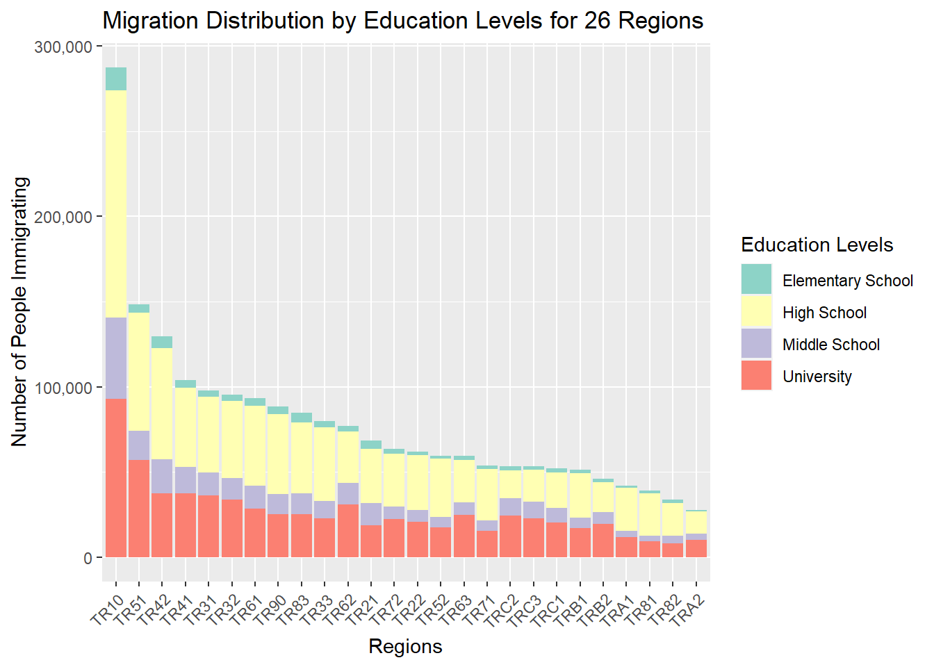
last_tidy_data_education2 <- tidy_literate|> pivot_longer(c(university,highschool,middleschool,elementaryedu,doctorate,primaryedu,master),names_to = "education",values_to = "education_value")

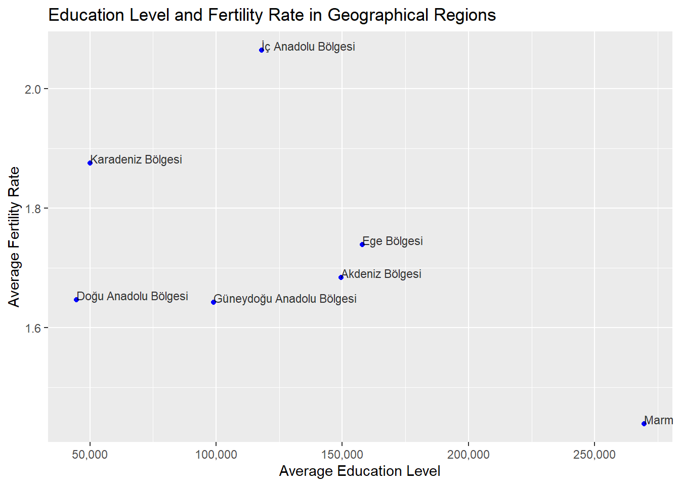
last_population_tidy_data <- last_tidy_data_education2 |> pivot_longer(c(fertilityrate,electricity,numberofattempts,housingsalesnumbers),names_to = "othervariables",values_to = "othervariables_value")
head(last_population_tidy_data)

# A tibble: 6 × 15
    IDD city  regionid regions         totalpop gender gender_value agerange
  <dbl> <chr> <chr>    <chr>              <dbl> <chr>         <dbl> <chr>   
1     1 Adana A        Akdeniz Bölgesi  2263373 male        1130862 age04   
2     1 Adana A        Akdeniz Bölgesi  2263373 male        1130862 age04   
3     1 Adana A        Akdeniz Bölgesi  2263373 male        1130862 age04   
4     1 Adana A        Akdeniz Bölgesi  2263373 male        1130862 age04   
5     1 Adana A        Akdeniz Bölgesi  2263373 male        1130862 age04   
6     1 Adana A        Akdeniz Bölgesi  2263373 male        1130862 age04   
# ℹ 7 more variables: agerange_value <dbl>, literate <chr>,
#   literate_values <dbl>, education <chr>, education_value <dbl>,
#   othervariables <chr>, othervariables_value <dbl>

Click the see the code

population$`region2id`<- ""
for (i in 1:nrow(population)) {
  city <- population$city[i]
  
  for (j in 1:length(region26$region)) {
    if (grepl(city, region26$region[j])) {
      population$`region2id`[i] <- paste(region26$`region2id`[j])
      break 
    }
  }
}

Now that all data preparations are complete, we can begin the process of visualization :)

DATA VISUALIZATION

Migration Causes VS. Migration Values

Click the see the code

library(tidyverse)
library(readxl)
library(readr)

# Migration Causes Box Plot
last_migration_tidy_data |> mutate(migrationcauses = reorder(migrationcauses, migrationcauses_value, FUN = median)) |>
  ggplot(aes(migrationcauses,migrationcauses_value,fill = migrationcauses)) +
  geom_boxplot() + ggtitle("Migration Causes") + xlab("Migration Causes") +
  ylab("Values") + theme(axis.text.x = element_text(angle= 90, hjust = 1)) + xlab("") +
  scale_y_continuous(trans = "log2") 

To have an overview of data on migration causes we plotted a box plot to see what reasons cause migration the most. Box plot shows that education is the most common reason for migration followed by migration due to a family member and better life conditions.

When plotting the box plot we scaled y values to log2 scale to see the distribution better and we ordered the box plots to make it easier to understand which are the most and the least causes of migration.

Regions and Reasons for Migration

Click the see the code

region_plot <- last_migration_tidy_data |> select(migrationcauses,migrationcauses_value,regions) |>
  ggplot(aes(migrationcauses,migrationcauses_value)) + geom_point(aes(color = regions)) +
  ggtitle("Regions and Reasons for Migration") + xlab("Migration Causes") +
  ylab("Migration Values") + theme(axis.text.x = element_text(angle= 90, hjust = 1)) + xlab("") + scale_y_continuous(trans = "log2")  
print(region_plot)

When we analyze migration reasons on a regional basis, we observe that under the category of ‘different reasons,’ the highest migration has occurred to the Marmara region. Following the Marmara region, the second-highest migration took place to the Central Anatolia region. This drew our attention to a few points. We had expected that the highest migration due to retirement would be to the Central Anatolian Region or Aegean Region, but it turned out that the majority of migration happened to the Marmara region.

Metropolitan Cities and Reasons for Migration

Click the see the code

city_plot <- last_migration_tidy_data |> filter(city %in% c("Ankara","İstanbul","İzmir","Antalya","Trabzon","Ağrı","Şanlıurfa")) |> select(migrationcauses,migrationcauses_value,city) |>
  ggplot(aes(migrationcauses,migrationcauses_value)) + geom_point(aes(color = city)) +
  ggtitle("Metropolitan Cities and Reasons for Migration") + xlab("Migration Causes") +
  ylab("Migration Values") + theme(axis.text.x = element_text(angle= 90, hjust = 1)) + xlab("") + scale_y_continuous(trans = "log2")  
print(city_plot)

While creating this graph, we included the most populous cities of each region because plotting for all 81 provinces would be quite challenging. As seen in this graph, the highest migration, due to different reasons, has been to Istanbul, followed by Ankara. What surprised us again is that the highest migration due to retirement is to İstanbul and Ankara.”

Regions and Migration Rates

Click the see the code

migration_gender2 <- last_migration_tidy_data |> mutate(rate = (last_migration_tidy_data$migrationcauses_value) / (last_migration_tidy_data$gender_value2))

region_rate_plot <- migration_gender2 |> ggplot(aes(migrationcauses,rate)) + geom_point(aes(color = regions)) +
  ggtitle("Regions and Migration Rates") + xlab("Migration Causes") +
  ylab("Migration Rates") + theme(axis.text.x = element_text(angle= 45, hjust = 1)) + xlab("") + scale_y_continuous(trans = "log2")
  print(region_rate_plot)

In the above plots , plotted values were migration values with respect to migration reason and we got some results that we were not expecting. To understand the situation deeply we plotted migration rates rather than migration values and result was more of what we were expected to see. For example migration due to retirement was actually occurring to Central Anatolian Region and Black Sea Region.

Metropolitan Cities and Migration Rates

Click the see the code

migration_gender2 <- last_migration_tidy_data |> mutate(rate = (last_migration_tidy_data$migrationcauses_value) / (last_migration_tidy_data$gender_value2))
city_rate_plot <- migration_gender2 |> filter(city %in% c("Ankara","İstanbul","İzmir","Antalya","Trabzon","Ağrı","Şanlıurfa")) |> ggplot(aes(migrationcauses,rate)) + geom_point(aes(color = city)) +
    ggtitle("Metropolitan Cities and Migration Rates") + xlab("Migration Causes") +
    ylab("Migration Rates") + theme(axis.text.x = element_text(angle= 45, hjust = 1)) + xlab("") + scale_y_continuous(trans = "log2")  
  print(city_rate_plot) 

In the same fashion, the city that people migrate the most due to retirement is Trabzon followed by İzmir and Ankara.

Immigration Data of Age Ranges

Click the see the code

last_migration_tidy_data |> mutate(agerange2 = reorder(agerange2, agerange_value2, FUN = median)) |>
  ggplot(aes(agerange2,agerange_value2,fill = agerange2)) +
  geom_boxplot() + ggtitle("Immigration Data of Age Ranges") + xlab("Age Ranges") +
  ylab("Values") + theme(axis.text.x = element_text(angle= 90, hjust = 1)) + xlab("") +
  scale_y_continuous(trans = "log2") 

When we look at the graph, we see that the age range of the people who migrate the most is 20-24. The 15-19 age range ranks second. The age range of people who migrate the least is observed to be 40-44. When we look at the Immigration Data of Age Ranges, we see that the most immigration age range is 20-24. We can say that education was the highest value among the reasons for immigration and this is consistent with this. Likewise, the second place is 15-19. It can be interpreted that high school students also migrate for education. “finjob” ranks in the middle list of reasons for migration. If we consider 25-29 as the age for finding a job, we can comment that people aged 25-29 do not migrate only for the purpose of finding a job. For example, they may have migrated due to better living conditions. When we look at the graph, we see that the migration age of 40-44 migrates the least compared to other ages. In our opinion, we can conclude from the graph that people who are used to a certain order no longer want change. According to the chart, 10-14 years old is the second to last migration age range. “familymig” ranked second among the reasons for migration. We can say that there is a contradiction here. We would have expected a higher number of people migrating for health reasons. Health is very important for everyone, but unfortunately health services are not developed everywhere. Health problems are a factor that can be seen in all age groups, so we would expect the values to be high.

Correlations Between Migration Reasons and Age Ranges.

Click the see the code

cor(last_migration_tidy_data$migrationcauses_value, last_migration_tidy_data$agerange_value2)

[1] 0.4977804

This value indicates a moderate positive relationship between migration reasons and age ranges.

Education Level and Fertility Rate in Geographical Regions

Click the see the code

library(tidyverse)
# Extracting necessary columns from the 'last_tidy_data_education2' dataset
data <- last_tidy_data_education2 %>%
  select(regions, education, education_value, fertilityrate) 
# Calculating average education and fertility rate per region
education_fertility <- data %>%
  group_by(regions) %>%
  summarise(
    avg_education = mean(education_value),  # Calculating the mean education value for each region
    avg_fertility = mean(fertilityrate)     # Calculating the mean fertility rate for each region
  )
# Creating a scatter plot to visualize the relationship between education level and fertility rate across regions
ggplot(education_fertility, aes(x = avg_education, y = avg_fertility, label = regions)) +
  geom_point(color = "blue") +  # Adding points to represent each region
  geom_text(hjust = 0, vjust = 0, size = 3, color = "black", alpha = 0.8) +  # Adding text labels for regions
  labs(
    title = "Education Level and Fertility Rate in Geographical Regions",  # Title of the plot
    x = "Average Education Level",  # X-axis label
    y = "Average Fertility Rate"     # Y-axis label
  ) +
  scale_x_continuous(labels = scales::comma, breaks = seq(0, 300000, by = 50000))  # Formatting X-axis labels

The scatter plot does not show a clear correlation between the average education level and fertility rate across regions. The points representing different regions are scattered without showing a clear trend of increase or decrease. The region with the highest average education level is Marmara, with about 250,000 units of education value. The region with the lowest average education level is Eastern Anatolia Region, with about 50,000 units of education value. The region with the highest average fertility rate is Central Anatolia Region, with above 2.0 children per woman. The region with the lowest average fertility rate is the Marmara Region, with below 1.5 children per woman. There are some outliers in the data, such as Central Anatolia Region, which has a relatively high average education level but also a high average fertility rate, and Mediterranean Region, which has a relatively low average education level but also a low average fertility rate. These outliers may indicate that there are other factors influencing the fertility rate besides the education level, such as culture, religion, income, etc. The surprising point in this data is that I expected the Eastern Anatolia Region to have the highest fertility rate. The low population registration rates in that region may be one of the reasons affecting the data output. According to TUIK data, the population registration rate of the Eastern Anatolia Region is 97.92%, which is 98.82% below the Turkey average. This may mean that some of the children born in this region are not registered.

Migration Distribution by Education Levels for 26 Regions

Click the see the code

library(tidyverse)
# Merging population and migration datasets based on the 'city' column
merged_data <- population %>%
  inner_join(migration, by = "city") %>%
  # Selecting specific columns from the merged dataset
  select(city, region2id, university2, highschool2, middleschool2, elementaryschool2)

# Transforming the merged data into a tidy format using pivot_longer
merged_data_tidy <- merged_data %>%
  pivot_longer(
    cols = c(university2, highschool2, middleschool2, elementaryschool2),
    names_to = "education_level",
    values_to = "migration_count"
  ) %>%
  # Grouping by region and education level to calculate total migration counts
  group_by(region2id, education_level) %>%
  summarise(total_migration = sum(migration_count, na.rm = TRUE)) %>%
  ungroup() %>%
  # Renaming education levels for better readability
  mutate(
    education_level = case_when(
      education_level == "university2" ~ "University",
      education_level == "middleschool2" ~ "Middle School",
      education_level == "highschool2" ~ "High School",
      education_level == "elementaryschool2" ~ "Elementary School",
      TRUE ~ as.character(education_level)
    )
  )  

# Sorting regions based on total migration counts
sorted_regions <- merged_data_tidy %>%
  group_by(region2id) %>%
  summarise(total_migration = sum(total_migration, na.rm = TRUE)) %>%
  arrange(desc(total_migration)) %>% 
  pull(region2id)

# Reordering factor levels of 'region2id' based on sorted regions
merged_data_tidy$region2id <- factor(merged_data_tidy$region2id, levels = sorted_regions)

# Creating a stacked bar plot to visualize migration distribution by education levels across regions
ggplot(merged_data_tidy, aes(x = region2id, y = total_migration, fill = education_level)) +
  geom_bar(stat = "identity", position = "stack") +  # Stacked bar plot
  labs(
    title = "Migration Distribution by Education Levels for 26 Regions",  # Title of the plot
    x = "Regions",  # X-axis label
    y = "Number of People Immigrating",  # Y-axis label
    fill = "Education Levels"  # Legend label
  ) +
  theme(axis.text.x = element_text(angle = 45, hjust = 1)) +  # Rotating x-axis labels for better readability
  scale_fill_brewer(palette = "Set3") +  # Setting color palette for education levels
  scale_y_continuous(labels = scales::comma)  # Formatting Y-axis labels using commas for better readability

It is seen that immigrants with high education levels mostly migrate to regions numbered TR10, TR51 and TR42. These regions cover the northwestern, western and southwestern regions of Turkey. It may indicate that these regions are more attractive in terms of education and job opportunities. It is seen that immigrants with low education level mostly migrate to TR81, TR82 and TRA2 regions. These regions cover the northeastern, eastern and southeastern regions of Turkey. It may indicate that these regions are poorer in terms of education and job opportunities. It may indicate that other Regions are average in terms of education and job opportunities.

Migration by Education Level

Click the see the code

library(tidyverse)

# Merging two datasets 'population' and 'migration' based on the common column 'city'
merged_data <- inner_join(population, migration, by = "city") %>%
  # Selecting specific columns from the merged dataset
  select(city, region2id, university2, doctorate, highschool2, elementaryschool2, middleschool2, finjob)

# Reshaping the data using pivot_longer to gather migration counts for different education levels
education_migration <- merged_data %>%
  pivot_longer(
    cols = c(university2, doctorate, highschool2, elementaryschool2, middleschool2),
    names_to = "education_level",
    values_to = "migration_count"
  ) %>%
  # Renaming and categorizing education levels for better visualization
  mutate(
    education_level = case_when(
      education_level == "university2" ~ "University",
      education_level == "doctorate" ~ "Doctorate",
      education_level == "highschool2" ~ "High School",
      education_level == "elementaryschool2" ~ "Elementary School",
      education_level == "middleschool2" ~ "Middle School",
      TRUE ~ as.character(education_level)
    )
  )

# Setting the order of the education levels for better visualization
education_migration$education_level <- factor(education_migration$education_level, 
                                             levels = c("Elementary School", "Middle School", "High School", "University", "Doctorate"))

# Creating a boxplot to visualize the migration count across different education levels
ggplot(education_migration, aes(x = education_level, y = migration_count, fill = education_level)) +
  geom_boxplot() +  # Adding boxplot geometry
  labs(
    title = "Migration by Education Level",  # Title of the plot
    x = "Education Level",  # X-axis label
    y = "Migration Count",  # Y-axis label
    fill = "Education Level"  # Legend label
  ) +
  theme_minimal() +  # Applying a minimal theme to the plot
  scale_y_continuous(trans = "log2" )  # Formatting Y-axis labels with commas for thousands

On the x axis, there are four education levels: doctorate, primary school, high school and university. On the Y axis, the number of people migrating is shown with values ranging from 0 to 100,000. In the graph, the number of migrations of individuals at doctoral or primary school level is much less than that of individuals at high school and university levels. In the graph, the highest number of migrations is seen among individuals at university level. This is followed by individuals at the high school level. It is seen that individuals with a higher level of education migrate less than individuals with a lower level of education. This may indicate that individuals with higher levels of education are more dependent on working conditions or find fewer job opportunities. It is seen that individuals with low education levels migrate more than individuals with high education levels. This may indicate that individuals with lower levels of education strive more to improve their living conditions or are under more pressure.

Inter-regional Rate Distributions

Click the see the code

migration_rate <- (migration$male2+migration$female2)/population$totalpop
numberofattempts_rate <- population$numberofattempts/population$totalpop
housingsalesnumbers_rate <- population$housingsalesnumbers/population$totalpop
electricity_rate <- population$electricity/population$totalpop
educated_rate <- (population$highschool + population$university + population$master + population$doctorate)/population$totalpop

merged_data <- cbind(population, numberofattempts_rate, housingsalesnumbers_rate, electricity_rate)

merged_data$regions <- factor(merged_data$regions) 




merged_data_long <- merged_data %>%
  pivot_longer(cols = c(numberofattempts_rate, housingsalesnumbers_rate, electricity_rate),
               names_to = "variable", values_to = "rate")


ggplot(merged_data_long, aes(x = regions, y = rate, fill = regions)) +
  geom_boxplot() +
  labs(x = "Regions", y = "Rate", title = "Interregional Rate Distributions") +
  facet_wrap(~ variable, scales = "free_y", ncol = 1) +
  theme(axis.text.x = element_text(angle = 45, hjust = 1))

Click the see the code

ratios <- data.frame(
  electricity_rate ,  
 housingsalesnumbers_rate,
  numberofattempts_rate,
  migration_rate,
 educated_rate
)

correlation_matrix <- cor(ratios)

print(correlation_matrix)

                         electricity_rate housingsalesnumbers_rate
electricity_rate                1.0000000                0.2673481
housingsalesnumbers_rate        0.2673481                1.0000000
numberofattempts_rate           0.4605411                0.4822953
migration_rate                  0.6837392                0.2184274
educated_rate                   0.6228220                0.2711951
                         numberofattempts_rate migration_rate educated_rate
electricity_rate                     0.4605411      0.6837392     0.6228220
housingsalesnumbers_rate             0.4822953      0.2184274     0.2711951
numberofattempts_rate                1.0000000      0.5059387     0.6996717
migration_rate                       0.5059387      1.0000000     0.8014049
educated_rate                        0.6996717      0.8014049     1.0000000

Click the see the code

population$`Migration Rate` <- (migration$male2 + migration$female2) / population$totalpop
population$`Number of Attempts Rate` <- population$numberofattempts / population$totalpop
population$`Housing Sales Numbers Rate` <- population$housingsalesnumbers / population$totalpop
population$`Electricity Rate` <- population$electricity / population$totalpop


rates_data <- population %>%
  select(city, region2id, `Migration Rate`, `Number of Attempts Rate`, `Housing Sales Numbers Rate`, `Electricity Rate`)

rates_data_tidy <- rates_data %>%
  pivot_longer(
    cols = c(`Migration Rate`, `Number of Attempts Rate`, `Housing Sales Numbers Rate`, `Electricity Rate`),
    names_to = "rate_type",
    values_to = "rate_value"
  )

ggplot(rates_data_tidy, aes(x = region2id, y = rate_value, fill = rate_type)) +
  geom_bar(stat = "identity", position = "stack") +
  labs(
    title = "Rates Distribution across Regions",
    x = "Regions",
    y = "Rate Value",
    fill = "Rate Types"
  ) +
  theme(axis.text.x = element_text(angle = 45, hjust = 50)) +
  scale_fill_brewer(palette = "Set3") +
  scale_y_continuous(labels = scales::comma)

The high education level of the Marmara Region may cause electricity consumption to be high in this region. However, other regions appear to have lower-than-expected electricity consumption. While high usage is expected due to illegal electricity use, especially in Eastern Anatolia, the data do not support this prediction.

Since the Aegean Region is a summer resort, it was expected that house sales would be high. The fact that Southeastern Anatolia has the lowest housing sales rates is an expected result due to the development level of the region.

Number of Initiatives and Touristic Regions: The fact that the Black Sea is a region with an unexpectedly high number of initiatives may be due to the fact that it is a touristic region. This supports our prediction, as the Aegean Region ranks second as a touristic region. It is relatively expected that Southeastern Anatolia has the lowest number of startups. The fact that the Black Sea is a region with an unexpectedly high number of initiatives may be due to the fact that it is a touristic region. This supports our prediction, as the Aegean Region ranks second as a touristic region. It is relatively expected that Southeastern Anatolia has the lowest number of startups.

When looking at correlation analyses, although the correlation between electricity consumption and migration rates has the highest value, this relationship cannot be said to be linear. The observed high value of the correlation between education level and electricity consumption (close to 1) supports that high education level may be related to electricity consumption. We obtained results that support our opinion stated in first sentence.

In the analyzes made on a regional basis, no significant relationship is seen. It is observed that each region is associated with different data sets at different levels compared to the other.

Workforce and Usable Income

Click the see the code

library(knitr)
tablool<- data.frame(region26$region,region26$region2id)
kable(head(tablool,26), align = "c") 

region26.region	region26.region2id
Adana, Mersin	TR62
Ağrı, Kars, Iğdır, Ardahan	TRA2
Ankara	TR51
Antalya, Isparta, Burdur	TR61
Aydın, Denizli, Muğla	TR32
Balıkesir, Çanakkale	TR22
Bursa, Eskişehir, Bilecik	TR41
Erzurum, Erzincan, Bayburt	TRA1
Gaziantep, Adıyaman, Kilis	TRC1
Hatay, Kahramanmaraş, Osmaniye	TR63
İstanbul	TR10
İzmir	TR31
Kastamonu, Çankırı, Sinop	TR82
Kayseri, Sivas, Yozgat	TR72
Kırıkkale, Aksaray, Niğde, Nevşehir, Kırşehir	TR71
Kocaeli, Sakarya, Düzce, Bolu, Yalova	TR42
Konya, Karaman	TR52
Malatya, Elazığ, Bingöl, Tunceli	TRB1
Manisa, Afyonkarahisar, Kütahya, Uşak	TR33
Mardin, Batman, Şırnak, Siirt	TRC3
Samsun, Tokat, Çorum, Amasya	TR83
Şanlıurfa, Diyarbakır	TRC2
Tekirdağ, Edirne, Kırklareli	TR21
Trabzon, Ordu, Giresun, Rize, Artvin, Gümüşhane	TR90
Van, Muş, Bitlis, Hakkari	TRB2
Zonguldak, Karabük, Bartın	TR81

Click the see the code

library(ggplot2)
ggplot(region26, aes(x = workforce15plus, y = usableincome, group = region2id)) + 
  geom_point(aes(color = region2id), size = 3) +
  labs(title = "Workforce vs Usable Income", x = "Workforce", y = "Usable Income")

We can see that TÜİK has divided our provinces into 26 regions and their code in the table. To understand and confirm this, we contacted TÜİK. As observed, the cities in the divided regions are close to each other. Over the phone, they responded that they based this division on the proximity, indicating, for instance, that the regional director in Van is also responsible for the work in other connected cities. Therefore, for ease of data collection, they adopted this method, as far as we understood.

Workforce and usable income graph shows us the relationship between workforce and usable income across different regions. Each colored dot represents a specific region and shows its usable income against the workforce. The table indicates that as the workforce increases, so does the usable income. However, it’s noteworthy that this increase is not uniform across all regions.

Usable income is presented through the Gini coefficient to measure income distribution within a region. The Gini coefficient is a number between 0 and 1, where 0 represents perfect equality, and 1 signifies perfect inequality. The higher the Gini coefficient, the greater the inequality. For instance, based on 2021 TÜİK data, the Gini coefficient in Istanbul is calculated as 0.43, whereas in Izmir, it stands at 0.37. According to this data, income inequality in Istanbul is higher than that in Izmir.

Click the see the code

cor(region26$usableincome, region26$workforce15plus)

[1] 0.5162115

Generally, a value between 0 and 0.3 indicates weak correlation, between 0.3 and 0.7 suggests a moderate level of correlation, and between 0.7 and 1 indicates a strong correlation. According to the result, there is a moderate positive relationship between workforce and usable income. With a correlation coefficient of 0.5162115, it indicates a linear relationship between workforce and usable income.