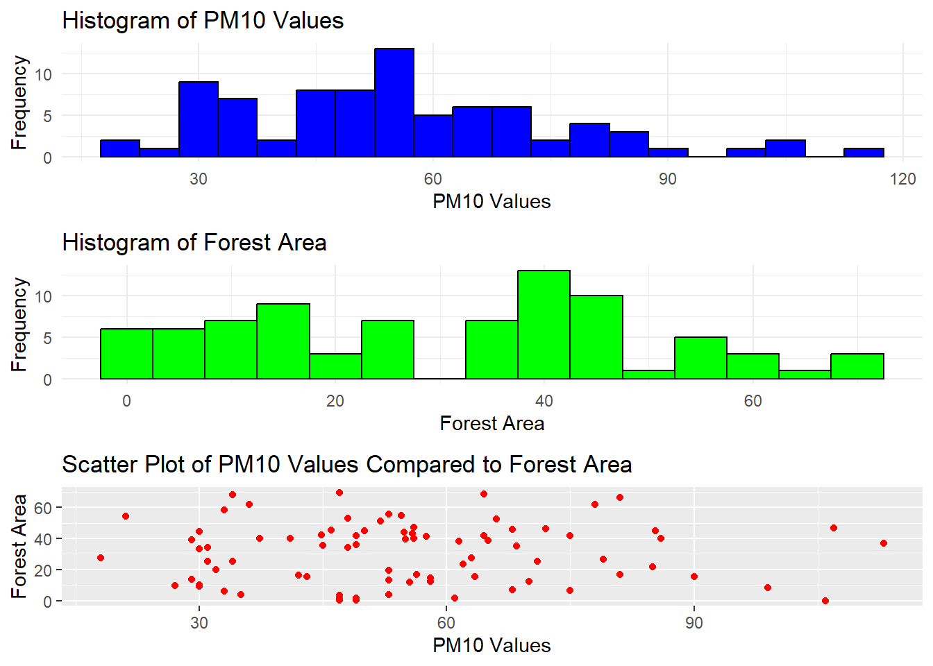
Our dataset consists of 3 columns. Provinces, pm10_values and forest area. Provinces are categorical variables representing the geographical location or provinces in Turkey, pm10_values are quantitative variables representing the average PM10 values, a common measure of air quality, higher values indicate higher levels of air pollution and forest_area values are quantitative variables representing the percentage of forest area per square kilometer. It reflects the extent of forest coverage in each province. The distribution of PM10 values across provinces can be visualized using a histogram. This would provide insights into the range and frequency of air pollution levels. The distribution of forest area percentages can be visualized using a histogram as well. This helps understand the variation in forest coverage among provinces. Correlation between PM10 values and forest area can be visually represented with a scatter plot. We can ompare provinces in different regions of Turkey to identify regional patterns in air pollution and forest area. A bar chart or grouped box plot can be useful for such comparisons.We can Rank provinces based on PM10 values and forest area to identify provinces with the highest and lowest values. This can be visualized using bar charts or a dual-axis plot.
Here is some additional analysis for our project ( we’ll be use provinces further in our analysis) :
library(ggplot2)
library(dplyr)
library(gridExtra)
# Librarieslibrary(ggplot2)
Warning: package 'ggplot2' was built under R version 4.3.2
library(dplyr)
Warning: package 'dplyr' was built under R version 4.3.2
Attaching package: 'dplyr'
The following objects are masked from 'package:stats':

    filter, lag
The following objects are masked from 'package:base':

    intersect, setdiff, setequal, union
library(gridExtra)
Warning: package 'gridExtra' was built under R version 4.3.2
Attaching package: 'gridExtra'
The following object is masked from 'package:dplyr':

    combine
data1 <-"https://raw.githubusercontent.com/emu-hacettepe-analytics/emu430-fall2023-team-alti_ustu_data/master/project_data.csv"project_data <-read.csv(data1)summary_data <- project_data %>%summarise(Avg_PM10 =mean(pm10_values),SD_PM10 =sd(pm10_values),Avg_Forest_Area =mean(forest_area),SD_Forest_Area =sd(forest_area) )p1 <-ggplot(project_data, aes(x = pm10_values)) +geom_histogram(binwidth =5, fill ="blue", color ="black") +theme_minimal() +labs(title ="Histogram of PM10 Values",x ="PM10 Values", y ="Frequency")p2 <-ggplot(project_data, aes(x = forest_area)) +geom_histogram(binwidth =5, fill ="green", color ="black") +theme_minimal() +labs(title ="Histogram of Forest Area",x ="Forest Area", y ="Frequency")p3 <-ggplot(project_data, aes(x = pm10_values, y = forest_area)) +geom_point(color ="red") +labs(title ="Scatter Plot of PM10 Values Compared to Forest Area",x ="PM10 Values", y ="Forest Area")grid.arrange(p1, p2, p3, ncol =1)
As you can see, contrary to our expectations, the PM10 values do not decrease as forest area increases. While in some places, the correlation might align with expectations, in most areas, there isn’t a clear inverse relationship. Drawing from some articles, we can explain the reasons as follows:
‘More forest means more pollen.’ Pollens contribute to the increase in PM10 levels. Thus, in cities with abundant forest areas, the rise in PM10 levels is attributed to this factor.
Particles resulting from forest fires increase PM10 levels. While forest density and forest fires may not follow a linear positive relationship, the likelihood of forest fires increases with forest density, potentially leading to an associated increase in PM10 levels.
***Emissions from vehicles increase PM10 levels. In a scenario with dense forest areas and heavy traffic, a proportional relationship between PM10 levels and forest area might be inevitable.
Even if the forest area is not dense, a natural environment less affected by human factors is expected to have lower PM10 levels.”
library(readxl)
Warning: package 'readxl' was built under R version 4.3.2
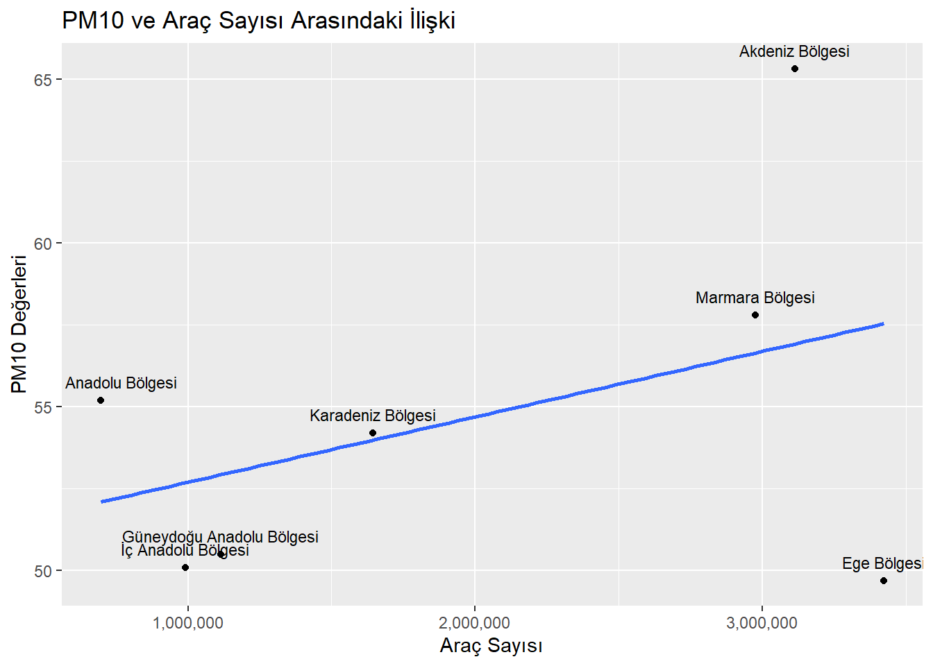
data2 <-"https://raw.githubusercontent.com/emu-hacettepe-analytics/emu430-fall2023-team-alti_ustu_data/master/bolgelerin_arac_sayilari_2015.csv"data2_cleaned <-read.csv(data2)bölgeler_arac_sayısı <-na.omit(data2_cleaned)corelation <-cor.test(bölgeler_arac_sayısı$toplam, bölgeler_arac_sayısı$PM10)ggplot(bölgeler_arac_sayısı, aes(x = toplam, y = PM10)) +geom_point() +geom_text(aes(label = Bölgeler), vjust =-1, size =3) +geom_smooth(method = lm, se =FALSE) +scale_x_continuous(labels = scales::comma) +labs(x ="Araç Sayısı", y ="PM10 Değerleri", title ="PM10 ve Araç Sayısı Arasındaki İlişki")
`geom_smooth()` using formula = 'y ~ x'
Slide Title: Impact of Vehicle Numbers on PM10 Pollution
“This plot correlates the number of vehicles to PM10 levels in Turkish regions. As vehicle numbers rise, so does PM10, indicating a direct link between traffic and air pollution.”
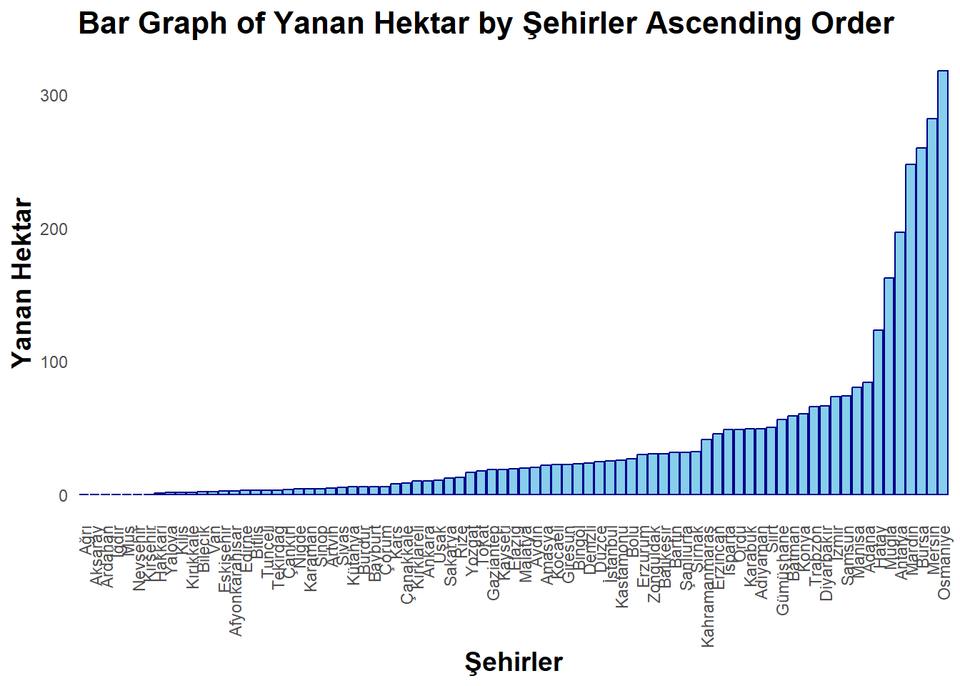
library(readxl)library(dplyr)library(ggplot2)library(scales)library(ggplot2)library(gridExtra)url<-"https://raw.githubusercontent.com/emu-hacettepe-analytics/emu430-fall2023-team-alti_ustu_data/master/firedata_csv.csv"data<-read.csv(url)data[data=="_"]=0data<- data %>%mutate(PM10.Values =ifelse(is.na(as.numeric(PM10.Values)), 0, as.numeric(PM10.Values)))data<- data %>%mutate(Yanan.Hektar.Hectare =ifelse(is.na(as.numeric(Yanan.Hektar.Hectare)), 0, as.numeric(Yanan.Hektar.Hectare)))data<- data %>%mutate(Yangın.Sayısı.Adet.Number. =ifelse(is.na(as.numeric(Yangın.Sayısı.Adet.Number.)), 0, as.numeric(Yangın.Sayısı.Adet.Number.)))cool_theme <-theme_minimal() +theme(panel.grid =element_blank(),axis.text.x =element_text(angle =90, vjust =0.5, hjust=1),plot.title =element_text(face ="bold", size =16),axis.title =element_text(face ="bold", size =14))p <-ggplot(data=data, aes(x =reorder(Şehirler, Yanan.Hektar.Hectare), y = Yanan.Hektar.Hectare)) +geom_bar(stat ="identity", fill ="skyblue", color ="darkblue") +labs(title ="Bar Graph of Yanan Hektar by Şehirler Ascending Order",x ="Şehirler",y ="Yanan Hektar") + cool_themeprint(p)
“This bar graph ranks cities by the extent of land burned, with the least affected on the left and the most on the right.”
library(readxl)library(dplyr)library(ggplot2)library(scales)library(ggplot2)library(gridExtra)url<-"https://raw.githubusercontent.com/emu-hacettepe-analytics/emu430-fall2023-team-alti_ustu_data/master/firedata_csv.csv"data<-read.csv(url)data[data=="_"]=0data<- data %>%mutate(PM10.Values =ifelse(is.na(as.numeric(PM10.Values)), 0, as.numeric(PM10.Values)))data<- data %>%mutate(Yanan.Hektar.Hectare =ifelse(is.na(as.numeric(Yanan.Hektar.Hectare)), 0, as.numeric(Yanan.Hektar.Hectare)))data<- data %>%mutate(Yangın.Sayısı.Adet.Number. =ifelse(is.na(as.numeric(Yangın.Sayısı.Adet.Number.)), 0, as.numeric(Yangın.Sayısı.Adet.Number.)))cool_theme <-theme_minimal() +theme(panel.grid =element_blank(),axis.text.x =element_text(angle =90, vjust =0.5, hjust=1),plot.title =element_text(face ="bold", size =16),axis.title =element_text(face ="bold", size =14))p <-ggplot(data=data, aes(x =factor(Şehirler, levels =unique(Şehirler)), y = Yanan.Hektar.Hectare)) +geom_bar(stat ="identity", fill ="skyblue", color ="darkblue") +labs(title ="Bar Graph of Yanan Hektar by Şehirler Alphabetical Order",x ="Şehirler",y ="Yanan Hektar") + cool_theme
“This bar chart orders cities alphabetically, showing varying levels of land burned in each city.”
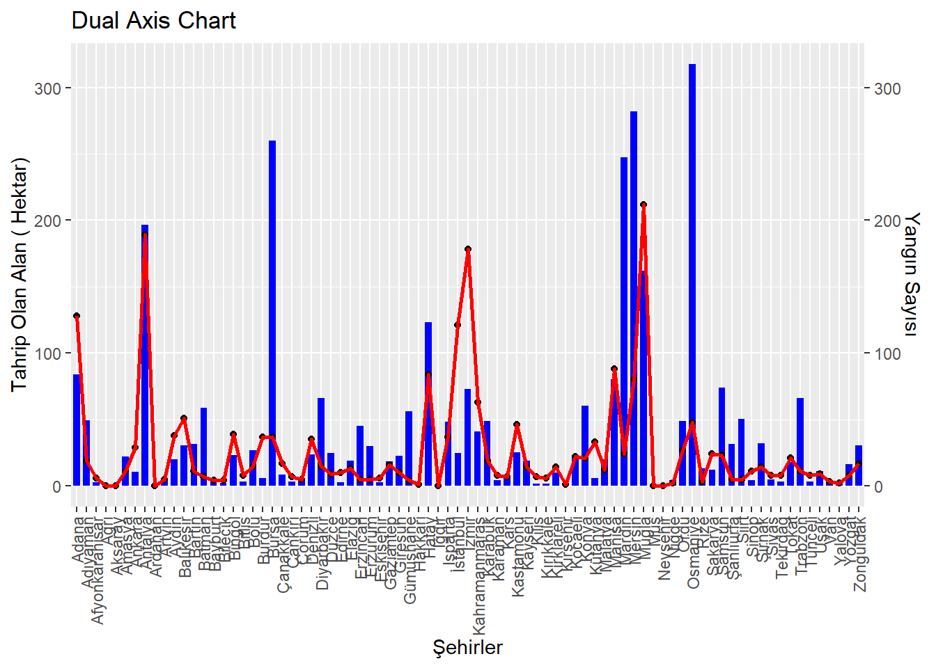
library(readxl)library(dplyr)library(ggplot2)library(scales)library(ggplot2)library(gridExtra)url<-"https://raw.githubusercontent.com/emu-hacettepe-analytics/emu430-fall2023-team-alti_ustu_data/master/firedata_csv.csv"data<-read.csv(url)data[data=="_"]=0data<- data %>%mutate(PM10.Values =ifelse(is.na(as.numeric(PM10.Values)), 0, as.numeric(PM10.Values)))data<- data %>%mutate(Yanan.Hektar.Hectare =ifelse(is.na(as.numeric(Yanan.Hektar.Hectare)), 0, as.numeric(Yanan.Hektar.Hectare)))data<- data %>%mutate(Yangın.Sayısı.Adet.Number. =ifelse(is.na(as.numeric(Yangın.Sayısı.Adet.Number.)), 0, as.numeric(Yangın.Sayısı.Adet.Number.)))ggplot(data=data, aes(x = Şehirler)) +geom_col(aes(y = Yanan.Hektar.Hectare), fill ='blue', width =0.7) +geom_point(aes(y = Yangın.Sayısı.Adet.Number.)) +geom_path(aes(y = Yangın.Sayısı.Adet.Number.), group =1, colour ="red", size =0.9) +scale_y_continuous(sec.axis =sec_axis(trans =~., name ="Yangın Sayısı")) +labs(title ="Dual Axis Chart", x ="Şehirler", y ="Tahrip Olan Alan ( Hektar)") +theme(axis.text.x =element_text(angle =90, hjust =1, vjust =0.5))
Warning: Using `size` aesthetic for lines was deprecated in ggplot2 3.4.0.
ℹ Please use `linewidth` instead.
“In this dual-axis chart, we’re looking at two related pieces of data across various cities. The red line graph shows the number of fire incidents, while the blue bars measure the actual damage caused by these fires, in hectares.
A quick observation reveals that higher frequencies of fires don’t always correspond to more extensive damage — some cities with fewer fires have experienced greater destruction, suggesting variability in fire severity or effectiveness of fire management strategies.
This data can inform emergency services, guiding resource allocation and prevention measures.”
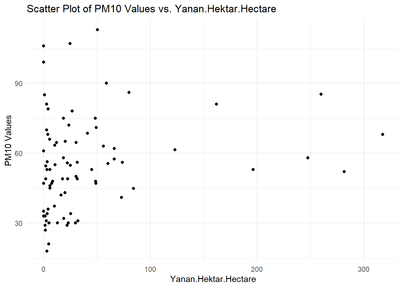
library(readxl)library(dplyr)library(ggplot2)library(scales)library(ggplot2)library(gridExtra)url<-"https://raw.githubusercontent.com/emu-hacettepe-analytics/emu430-fall2023-team-alti_ustu_data/master/firedata_csv.csv"data<-read.csv(url)data[data=="_"]=0data<- data %>%mutate(PM10.Values =ifelse(is.na(as.numeric(PM10.Values)), 0, as.numeric(PM10.Values)))data<- data %>%mutate(Yanan.Hektar.Hectare =ifelse(is.na(as.numeric(Yanan.Hektar.Hectare)), 0, as.numeric(Yanan.Hektar.Hectare)))data<- data %>%mutate(Yangın.Sayısı.Adet.Number. =ifelse(is.na(as.numeric(Yangın.Sayısı.Adet.Number.)), 0, as.numeric(Yangın.Sayısı.Adet.Number.)))data_sorted <- data[order(data$Yanan.Hektar.Hectare), ]ggplot(data_sorted, aes(x = Yanan.Hektar.Hectare, y = PM10.Values)) +geom_point() +labs(title ="Scatter Plot of PM10 Values vs. Yanan.Hektar.Hectare",x ="Yanan.Hektar.Hectare", y ="PM10 Values") +theme_minimal()
“This scatter plot maps the relationship between PM10 air pollution levels and the area of land burned, measured in hectares. There’s no clear correlation visible from the data points; however, most instances of higher PM10 values do not necessarily coincide with larger burned areas. This suggests that factors other than air pollution may play a more significant role in the extent of land affected by fires.”